

1. Introduction
- RPS was commissioned by Berwick Bank Wind Farm Limited (BBWFL), a wholly owned subsidiary of SSE Renewables (SSER) Limited (hereafter ‘the Applicant’) to undertake a benthic subtidal and intertidal ecology characterisation of the Berwick Bank Wind Farm (hereafter referred to as “the Proposed Development”), and surrounding area to inform the Environmental Impact Assessment (EIA) Report. The Proposed Development array area is located in the outer Firth of Forth and Firth of Tay, 37.8 km east of the Scottish Borders coastline (St Abb’s Head) and 47.6 km to the East Lothian coastline from the nearest boundary. It covers an area of approximately 1,178.1 km2. Up to eight export cables will connect the Proposed Development to the mainland, via a cable landfall. The export cables which form part of the Proposed Development will make landfall on the East Lothian coast, specifically at Skateraw Harbour (hereafter referred to as the ‘Skateraw landfall’). From here, the Project will connect to a Scottish Power Energy Networks (SPEN) Transmission 400kV Grid Substation located at Branxton, which is located southeast of Torness Power station.
- This Benthic Subtidal and Intertidal Ecology Technical Report provides an up-to-date benthic subtidal and intertidal ecology baseline characterisation for the Proposed Development using the most recent desktop data and site-specific survey data.
- This report is structured as follows:
- section 2 - study area;
- section 3 – methodology and baseline characterisation, including details of desk-based sources and site-specific survey data; and
- section 4 – summary, including identification of Important Ecological Features (IEFs).
2. Study Area
2. Study Area
- For the purposes of the benthic subtidal and intertidal ecology assessment, two study areas have been defined:
- The Proposed Development benthic subtidal and intertidal ecology study area has been defined with reference to the Proposed Development boundary that existed prior to the boundary refinement in June 2022. As the refinements resulted in a reduction of the Proposed Development array area, the benthic subtidal and intertidal ecology study area is considered to remain representative and presents a conservative baseline against which the benthic and subtidal ecology assessment is undertaken. The Proposed Development benthic subtidal and intertidal ecology study area has not therefore been realigned to the current Proposed Development boundary. This includes intertidal habitats within the Proposed Development export cable corridor (between Mean Low Water Springs (MLWS) and Mean High Water Springs (MHWS) mark). It is the area within which the site specific benthic subtidal and intertidal surveys were undertaken ( Figure 2.1 Open ▸ ). Data collected from areas outside the Proposed Development benthic subtidal and intertidal ecology study area were analysed and included in the baseline characterisation as they provide further context to the data collected within the Proposed Development benthic subtidal and intertidal ecology study area.
- The regional benthic subtidal and intertidal ecology study area encompasses the wider northern North Sea habitats and includes the neighbouring consented offshore wind farms (and their associated export cable corridors) and designated sites ( Figure 2.1 Open ▸ ). It has been characterised by desktop data and provides a wider context to the site-specific data.
Figure 2.1: Benthic Subtidal and Intertidal Ecology Study Areas
3. Baseline
3. Baseline
3.1. Methodology
3.1. Methodology
- A desktop review has been undertaken to inform the baseline for benthic subtidal and intertidal ecology, including a review of a number of academic reports, reports from surveys undertaken to support other project consents and surveys to support the designation of Marine Protection Areas (MPAs) for offshore habitats located in the vicinity of the Proposed Development ( Table 3.1 Open ▸ ). These provide further context to the site-specific surveys ( Table 3.2 Open ▸ ).
- A benthic subtidal survey and a benthic intertidal survey have been undertaken to characterise the Proposed Development benthic subtidal and intertidal ecology study area for the purposes of informing the benthic subtidal and intertidal ecology EIA Report (volume 2, chapter 8). The subtidal ecology survey consisted of grab sampling, drop down video (DDV) sampling and epibenthic trawls. Analysis of results included multivariate and univariate statistical analyses as well as descriptions of the raw data. Data collection and analysis to inform various site-selection options resulted in areas being analysed that ultimately did not fall within the Proposed Development, however they have been included to provide further context.
- The intertidal survey involved a Phase 1 walkover and sediment sampling at the proposed landfall location. Detailed notes were taken along with waypoint locations at habitat changes and photographs of the habitats. These were reviewed to provide a biotope map of the proposed landfall location.
- Detailed methodologies for each survey are presented in section 3.4.
3.2. Desktop Study
3.2. Desktop Study
- Information on benthic subtidal and intertidal ecology within the regional benthic subtidal and intertidal ecology study area and the Proposed Development benthic subtidal and intertidal ecology study area was collected through a detailed desktop review of existing studies and datasets. These are summarised in Table 3.1 Open ▸ .
Table 3.1: Summary of Key Desktop Reports
3.2.1. Regional Benthic Subtidal and Intertidal Ecology Study Area
Subtidal sediments
- The seabed sediments of the regional benthic subtidal and intertidal ecology study area have been recorded as being dominated by circalittoral sand with patches of circalittoral coarse sediment, which is characteristic of the North Sea (EMODnet, 2019). The EMODnet (European Marine Observation and Data Network) broad-scale seabed habitat map for Europe (EUSeaMap) and the Marine Scotland National Marine Plan Interactive (NMPI) map present the European Nature Information System (EUNIS) habitat classifications for the northern North Sea ( Figure 3.1 Open ▸ ). The most common sediment types noted in the regional benthic subtidal and intertidal ecology study area were deep circalittoral sand, followed by deep circalittoral coarse sediment and deep circalittoral mud ( Figure 3.1 Open ▸ ), all identified as low energy habitats by EMODnet, 2019. Based on the EUSeaMap data, regions of higher topography and those associated with the bank complexes within the Firth of Forth approaches were dominated by deep circalittoral coarse sediments whereas those in deeper water and in the flanks of the banks were dominated by deep circalittoral sands ( Figure 3.1 Open ▸ ). Finer sediments were recorded in the nearshore areas of the regional benthic subtidal and intertidal ecology study area. There were large areas of circalittoral fine sand or circalittoral muddy sand, deep circalittoral mud and circalittoral sandy mud recorded at the entrance to the Firth of Forth and Firth of Tay. Further inshore, these fine sediments give way to moderate energy circalittoral rock, mixed and coarse sediments ( Figure 3.1 Open ▸ ; EMODnet, 2019).
- The Firth of Forth Banks Complex (FFBC) MPA has been strongly influenced by water currents with a mosaic of different types of sand and gravels, which create a unique range of habitats (JNCC, 2021a). Although these sediments were found to be relatively common around Scotland, the dynamic currents in the Firth of Forth Banks area influence the distribution of the sands and gravels (JNCC, 2014a). Axelsson et al. (2014) analysis of the video and still photography from surveys within the FFBC MPA undertaken in 2011 as part of the Scottish MPA Project, reported three broad habitat types: soft sediments with ripples; mixed sediment; and coarse sediments with some rocky outcrops. Gravelly sand sediments were more frequently recorded towards the north of the FFBC MPA with gravelly muddy sands and mixed sediments present to the south and west of the FFBC MPA (Axelsson et al., 2014). Acoustic data from surveys within the FFBC MPA undertaken in 2011 as part of the same project, reported sandy gravel, sand, gravelly sand and slightly gravelly sand in the approaches to the Firth of Forth and Wee Bankie to Gourdon areas (Sotheran and Crawford-Avis, 2013).
- The Wee Bankie moraine formation feature of the FFBC MPA occurs within the regional benthic subtidal and intertidal ecology study area. A large proportion of the Wee Bankie moraine formation can be found within the Wee Bankie (including Scalp Bank) part of the FFBC MPA and is considered to be a Key Geodiversity Area in Scotland’s seas. This formation comprised a series of prominent (20 m high) submarine glacial ridges, composed of poorly sorted sediments (boulders, gravels, sands and clays) (JNCC, 2020a). Brooks et al. (2013) regarded the moraine geodiversity features as being scientifically important due to their key role in improving our understanding of the glacial retreat history of the last British Irish ice sheet.
- The surveys conducted in 2011 to support the EIA benthic baseline characterisation for what were known at the time as the Seagreen Alpha/Bravo offshore wind farms (located immediately to the north of the Proposed Development array area, Figure 3.2 Open ▸ ) also provided an overview of the sedimentary habitats present within the regional benthic subtidal and intertidal ecology study area. In 2018, the Seagreen Alpha and Bravo projects were combined to form Seagreen in the same sea-area, which now comprises the Seagreen 1 and Seagreen Project 1A. This report refers to the superseded Seagreen (Alpha) and (Bravo) projects which were under development when the survey data was collected. The sediments present across the Seagreen (Alpha) array area ranged from cobbles with sand and gravelly sand in the west, to sandy gravel in the east. There was a greater predominance of fine sediments recorded across the Seagreen (Bravo) array compared with Seagreen (Alpha) array area, with sediments ranging from slightly gravelly sand in the west, sandy gravel in the central section and gravelly sand in the east of the Seagreen (Bravo) offshore wind farm. The majority of the seabed across both the Seagreen (Alpha and Bravo) array areas was level or undulating with occasional linear sediment waves (Seagreen, 2012).
- The baseline characterisation surveys for the nearby Inch Cape offshore wind farm array area (Inch Cape Offshore Limited, 2011) reported the sediments to be characterised primarily by circalittoral sands and gravelly sands, with smaller areas of muddy mixed sediment.
- The nearshore subtidal zone from North Berwick in Lothian to Flamborough Head in the East Riding of Yorkshire has been studied as part of the MNCR. Seabed sediments recorded in the nearshore subtidal zone of the regional benthic subtidal and intertidal ecology study area were sublittoral muddy sands, sublittoral fine sand, circalittoral rock and small areas of circalittoral mixed sediments (Brazier et al., 1998). The sediments recorded in the nearshore subtidal zone near the proposed landfall location were kelp forest with red algae and mobile sand shores (Brazier et al., 1998). The coastline at the Skateraw proposed landfall has experienced small amounts of accretion across the last 100 years (The Scottish Government, 2017).
Figure 3.1: Benthic Habitats (EMODNet, 2019) within the Regional Benthic Subtidal and Intertidal Ecology Study Area
Subtidal benthic ecology
- Cooper and Barry (2017) described the results of a baseline assessment of the UK’s subtidal macrobenthic infauna, with a particular focus around sites and regions of marine aggregate dredging. Although aggregates were the focus of the study, a “big data” approach was taken, collating data from across UK waters from various industries including offshore wind farms, oil and gas, nuclear and port and harbour sectors. This also included samples from the Neart na Gaoithe wind farm, within the regional benthic subtidal and intertidal ecology study area. Benthic infaunal communities were reported to be mainly polychaete and bivalve rich communities.
- The northern North Sea contains a variety of benthic ecology habitats but is mainly characterised by polychaete dominated communities (Spionidae, Glyceridae, Terebellidae, Capitellidae, Phyllodocidae and Nemertea), sparse faunal communities (Nephtyidae, Spionidae, Opheliidae) and diverse faunal communities (including the polychaetes: Spionidae, Nephtyidae, Lumbrineridae, Oweniidae, Cirratulidae, Capitellidae, Ampharetidae, the echinoderm Amphiuridae, the bivalve Semelidae and Nemertea) (Cooper and Barry, 2017).
- The MNCR study of the nearshore subtidal zone from North Berwick in Lothian to Flamborough Head in Yorkshire recorded nearshore seabed habitats in the regional benthic subtidal and intertidal ecology study area. Five seabed habitats were recorded (Brazier et al., 1998):
- SS.SMx.CMx.MysThyMx/SS.SMu.CSaMu.AfilMysAnit: Sublittoral muddy sand with echinoderms;
- IR.MIR.KR.Lhyp.Ft: Kelp forest with red algae;
- LS.LSa.MoSa.AmSco: Mobile sand shores with amphipods and polychaetes;
- SS.SSa.IFiSa.NcirBat: Sublittoral fine sand with polychaetes and bivalves; and
- CR.MCR.EcCr.FaAlCr.Bri: Circalittoral rock with brittlestars and hydroids.
- Analysis was undertaken on the data from seabed acoustic surveys that were carried out in 2013 to contribute to the evidence base for the presence and extent of MPA search features in Scottish waters (Southeran and Crawford-Avis, 2013). Phase 1 of the MPA search project surveys included the approaches to the Firth of Forth which overlaps with the regional benthic subtidal and intertidal ecology study area. Habitats ranged from sand sediments to coarse and mixed sediments in the inshore regions, and back to sand sediments in the offshore region. The biotope SS.SSa.CMuSa Circalittoral muddy sand was recorded in the nearshore subtidal area close to St. Andrews with circalittoral rock habitats, CR.HCR.XFa Mixed faunal turf communities/CR.MCR.EcCr Echinoderms and crustose communities recorded in the nearshore subtidal area off Craighead. SS.SSa.OSa Offshore subtidal sand was recorded across the approaches to the Firth of Forth and the Wee Bankie to Gourdon areas however it was more frequently recorded in the regions further offshore. SS.SCS.OSC Offshore circalittoral coarse sediment was also recorded across the approaches to the Firth of Forth and Wee Bankie to Gourdon areas. SS.SMx.CMx Circalittoral mixed sediments and SS.SMx.OMx Offshore mixed sediments were recorded in areas further inshore. Occasional patches of circalittoral rock were also recorded across the approaches to the Firth of Forth and Wee Bankie to Gourdon areas (Southeran and Crawford-Avis, 2013).
- The following biotopes were reported within the regional benthic subtidal and intertidal ecology study area (Southeran and Crawford-Avis, 2013):
- kelp with cushion fauna and/or foliose red seaweeds: IR.HIR.KFaR.FoR.Dic Foliose red seaweeds with dense Dictyota dichotoma and/or Dictyopteris membranacea on exposed lower infralittoral rock/IR.HIR.KFaR.LhypRVt Laminaria hyperborea and red seaweeds on exposed vertical rock;
- mixed faunal turf communities on circalittoral rock: CR.HCR.XFa.FluCoAs.X Flustra foliacea and colonial ascidians on tide-swept exposed circalittoral mixed substrata/CR.HCR.XFa.FluCoAs.SmAs Flustra foliacea, small solitary and colonial ascidians on tide-swept circalittoral bedrock or boulders/CR.HCR.XFa.FluCoAs Flustra foliacea and colonial ascidians on tide-swept moderately wave-exposed circalittoral rock;
- circalittoral coarse sediment: SS.SCS.CCS.PomB Pomatoceros triqueter with barnacles and bryozoan crusts on unstable circalittoral cobbles and pebbles/SS.SCS.CCS;
- deep circalittoral coarse sediment: SS.SCS.OCS/SS.SCS.OCS.(PoGintBy)/SS.SCS.OCS.(Sbom);
- circalittoral muddy sand: SS.SSa.CMuSa.AalbNuc Abra alba and Nucula nitidosa in circalittoral muddy sand or slightly mixed sediment/SS.SSa.CMuSa;
- deep circalittoral sand: SS.SSa.OSa/SS.SSa.OSa.(Sbom);
- circalittoral mixed sediments: SS.SMx.CMx.OphMx Ophiothrix fragilis and/or Ophiocomina nigra brittlestar beds on sublittoral mixed sediment/SS.SMx.CMx.(FluHyd)/SS.SMx.CMx.MysThyMx Mysella bidentata and Thyasira spp. in circalittoral muddy mixed sediment/SS.SBR.PoR.SspiMx Sabellaria spinulosa on stable circalittoral mixed sediment;
- deep circalittoral mixed sediments: SS.SMx.OMx.(PoGintBy);
- SS.SBR.SMus.ModMx: Modiolus beds on open coast circalittoral mixed sediment;
- CR.MCR.EcCr.FaAlCr.Adig Alcyonium digitatum, Pomatoceros triqueter, algal and bryozoan crusts on wave-exposed circalittoral rock/CR.MCR.EcCr.FaAlCr.Flu Flustra foliacea on slightly scoured silty circalittoral rock; and
- SS.SMu.CFiMu.SpnMeg: Seapens and burrowing megafauna in circalittoral fine mud.
- Phase 2 of the MPA Project survey focused on the data from seabed acoustic surveys on the eastern approaches to the Firth of Forth, the western tip of which overlaps with the regional benthic subtidal and intertidal study area (Southeran and Crawford-Avis, 2014). The following biotopes were reported within the eastern approaches to the Firth of Forth area:
- SS.SCS.CCS: Circalittoral coarse sediment/deep circalittoral coarse sediment;
- SS.SSa.CMuSa: Circalittoral muddy sand; and
- SS.SSa.OSa: Deep circalittoral sand.
- With regards to protected species, the National Biodiversity Network (NBN) Atlas and the SeaSearch database include records of Sabellaria spp. and ocean quahog Arctica islandica in the regional benthic subtidal and intertidal ecology study area (NBN, 2021). NatureScot publications have been searched to understand the presence of Scottish PMFs in the regional benthic subtidal and intertidal ecology study area. Tyler-Walters et al., (2016) reported blue mussel (Mytilus edulis) and horse mussel (Modiolus modiolus) beds, burrowed mud, kelp beds, ocean quahog A. islandica aggregations, maerl or coarse shell gravel with burrowing sea cucumbers, seagrass beds and offshore subtidal sands and gravels within the regional benthic subtidal and intertidal ecology study area.
- S. spinulosa has been recorded within the regional benthic subtidal and intertidal ecology study area. S. spinulosa records in Scotland are limited to Lue Bay, the Solway Firth and the North Sea of Rattray Head. There are very few records of S. spinulosa from Scotland and even fewer extant records of reefs. This is thought to be due to low sampling effort to date and therefore it is expected that more records of species and reefs will be made as the offshore industry progresses in the region (Pearce and Kimber, 2020).
Seagreen Alpha/Bravo offshore wind farm
- The Seagreen Alpha/Bravo baseline characterisation surveys conducted in 2011 comprised infaunal grab sampling, beam trawl sampling and DDV sampling. The benthic habitats mapped for the EIA characterisation were divided into the following benthic community classes for each site:
Seagreen (Alpha) wind farm:
- western area: ‘Sabellaria’ (SS.SBR.PoR.SspiMx), ‘sparse polychaetes and bivalves’ (SS.SCS.ICS.MoeVen) and ‘faunal turf’ (SS.SMX.CMx.FluHyd); and
- central and eastern areas: dominated by the sabellid polychaete classes, ‘dense Chone’ (SS.SMx.OMx.(Chone)) and ‘sparse Chone’.
Seagreen (Bravo) wind farm:
- western half: ‘Sabellaria’, ‘rich polychaetes and bivalves’ and ‘epifauna with polychaetes’ (SS.SMx.OMx.PoVen); and
- eastern half: ‘dense Chone’ and ‘rich polychaetes’ (SS.SMx.OMx.PoVen).
- There was a clear divide between the two areas however ‘polychaete and bivalve’ habitats were also present in the most northern part of the eastern section of Seagreen (Bravo). There was also a patch of raised sandy gravel characterised by the brittlestar ‘Ophiothrix spp.’ (SS.SMx.CMx.OphMx) habitats located on or near the boundary between the western, central and eastern areas of Seagreen (Bravo).
- The number of species and individuals within the Seagreen (Bravo) wind farm site was generally lower than within the Seagreen (Alpha) wind farm site, which was likely to be a result of a predominance of finer sediments in the Seagreen (Bravo) wind farm site. Epifauna and encrusting fauna were common where the sediment contained gravel, shell or cobble. The distribution of epifauna was related to sediment type, with sandy gravels and gravelly sands supporting rich epifauna while gravelly sands were low in epifauna (Seagreen, 2012).
- High species richness was recorded in association with areas of Sabellaria habitat, although there was no evidence from the DDV surveys of extensive or well developed aggregations of Sabellaria within the Seagreen (Alpha) or Seagreen (Bravo) wind farm survey areas (Seagreen, 2012).
- Pre-construction benthic monitoring and Annex I reef surveys within the Seagreen array areas and export cable corridor were undertaken in 2020. Benthic habitats were recorded as circalittoral mixed sediments, SS.SMx.CMx.FluHyd and SS.SMx.CMx.OphMx, with patches of moderate energy circalittoral rock and circalittoral coarse sediment (APEM, 2020). The Annex I reef assessment reported that biogenic reefs (e.g. Annex 1 Sabellaria) were not present at any locations. Patches of medium resemblance stony reef were recorded among larger areas of cobble and sand in the export cable corridor, close to the Seagreen array area and within the north-east of the Seagreen array area. Patches of low resemblance stony reef were recorded in the export cable corridor, close to the Seagreen array area and within the north-east and central areas of the Seagreen array area (APEM, 2020). This is in line with the habitats mapped in the baseline characterisation presented in the Environmental Statement (Seagreen, 2012).
- A benthic validation survey was undertaken in 2020 and 2021 to support the marine licence application for an additional export cable corridor for Seagreen Project 1A ( Figure 3.2 Open ▸ ). The benthic subtidal survey comprised grab and DDV sampling and was undertaken to the north and north-west of the Proposed Development array area and around the subtidal areas off North Berwick. Sediments recorded ranged from sand to mixed sediments with sample stations closer to the coast containing a higher percentage of mud and those further offshore containing a higher percentage of sand. The Seagreen (Alpha) benthic validation survey recorded sandy mud biotopes (SS.SMu.CSaMu and SS.SMu.CSaMu.AfilMysAnit Amphiura filiformis, Mysella bidentata and Abra nitida in circalittoral sandy mud) across the mid-section of the export cable corridor survey area. Mixed sediment biotopes (SS.SMx.OMx.PoVen Polychaete-rich deep Venus community in offshore mixed sediments and SS.SMx.OMx.OphMx) were recorded in the furthest offshore samples within the export cable corridor survey area. The inshore sections of the export cable corridor survey area were dominated by muddy sediment biotopes (SS.SMu.CFiMu.SpnMeg and SS.SMu.ISaMu.MelMagThy Melinna palmata with Magelona spp. and Thyasira spp. in infralittoral sandy mud). The Seagreen (Alpha) benthic validation survey recorded SS.SMu.CSaMu.AfilMysAnit, SS.SMu.CSaMu, SS.SMx.OMx.PoVen and SS.SMx.OMx.OphMx overlapping with the north-west corner of the Proposed Development array area ( Figure 3.2 Open ▸ ). No Annex I reefs were recorded during the Seagreen (Alpha) benthic validation surveys.
Inch Cape offshore wind farm
- The Inch Cape wind farm is located 7.7 km to the west of the Proposed Development and within the regional benthic subtidal and intertidal ecology study area ( Figure 3.2 Open ▸ ). The baseline characterisation surveys for the Inch Cape wind farm showed that the array area was dominated by circalittoral sands and gravelly sands with areas of mixed sediment. The epifaunal surveys recorded epibenthic species that were typical for these sediments and included dead man’s fingers (Alcyonium digitatum), horned wrack (Flustra foliacea), brittlestar (Ophiothrix fragilis), hydroids (e.g. Hydrallmania falcata) and a number of small fish and mobile benthic invertebrates. The DDV survey recorded a number of similar species; the key species recorded were: A. digitatum, Pomatoceros triqueter, Munida rugosa, F. foliacea, and Asterias rubens. The brittlestar O. fragilis occurred in high densities, but only at two stations (Inch Cape Offshore Limited, 2011).
- The dominating biotopes within the array were SS.SMx.CMx.MysThyMx covering 65% of the array area, SS.SCS.OCS covering 31% of the area and SS.SCS.CCS.MedLumVen Mediomastus fragilis, Lumbrineris spp. and venerid bivalves in circalittoral coarse sand or gravel covering 4% of the area (Inch Cape Offshore Limited, 2011). A number of reef forming polychaetes (i.e. Sabellaria) were recorded; however, no evidence of Annex I reef features were recorded.
Neart na Gaoithe offshore wind farm
- The Neart na Gaoithe array area is approximately 16.3 km west of the Proposed Development and within the regional benthic subtidal and intertidal ecology study area ( Figure 3.2 Open ▸ ). The baseline characterisation surveys for the Neart na Gaoithe array area reported slightly gravelly sands with areas of coarser sediments (e.g. sandy gravels and gravelly sand). Analysis of the grab samples mainly characterised the array area as SS.SMu.CSaMu.AfilNten Amphiura filiformis and Nuculoma tenuis in circalittoral and offshore sandy mud and a mosaic of SS.SCS.CCS/SS.SSa.OSa. Small patches of SS.SMu.CSaMu.ThyNten were reported in the east, SS.SSa.CFiSa.ApriBatPo Abra prismatica, Bathyporeia elegans and polychaetes in circalittoral fine sand in the south and SS.SSa.OSa.OfusAfil Owenia fusiformis and Amphiura filiformis in offshore circalittoral sand or muddy sand in the north and west of the array area (EMU, 2010). No protected or rara species were recorded (EMU, 2010).
- Analysis of the DDV data mainly characterised the array area as SS.SMu.CFiMu.SpnMeg with regular patches of SS.SMx.CMx throughout the array area. SS.SMx Sublittoral mixed sediments, SS.SMx.CMx.OphMx and CR.MCR.EcCr (on boulders) were also recorded in small patches in the array area (EMU, 2010).
Figure 3.2: Offshore Wind Farms in the Regional Benthic Subtidal and Intertidal Ecology Study Area
3.2.2. Proposed Development Benthic Subtidal and Intertidal Study Area
Subtidal sediments
- Based on the EUSeaMap data, seabed sediments of the Proposed Development benthic subtidal and intertidal ecology study area have been recorded as being dominated by low energy deep circalittoral sand and low energy deep circalittoral coarse sediment (EMODnet, 2019). Deep circalittoral sands have been recorded in the offshore section of the export cable corridor with sediments becoming more variable in the inshore section of the export cable corridor; circalittoral sand sediments grade into deep circalittoral muds, deep circalittoral mixed sediments and deep circalittoral coarse sediments with increasing proximity to the landfall. Discrete areas of faunal communities on deep low energy circalittoral rock have been recorded throughout the inshore regions of the export cable corridor ( Figure 3.1 Open ▸ ).
- The Proposed Development benthic subtidal and intertidal ecology study area overlaps with the FFBC MPA, designated for offshore subtidal sands and gravels, shelf banks and mounds, and moraines representative of the Wee Bankie Key Geodiversity Area (JNCC, 2021a). The FFBC MPA comprises the large-scale morphological bank features Berwick, Scalp and Montrose Banks and the Wee Bankie ( Figure 3.1 Open ▸ ). The Proposed Development overlaps the Berwick Bank and the southern section of the Scalp Bank and Wee Bankie aspects of the FFBC MPA. Habitat maps (Sotheran and Crawford-Avis, 2013 and 2014) and biotope assignment of 2011 still and grab sample data (Axelsson et al., 2014; Pearce et al., 2014) reported offshore subtidal sand and gravel habitats in the FFBC MPA. Axelsson et al. (2014) reported gravelly muddy sands and sands within the area overlapping the Proposed Development array area.
Subtidal benthic ecology
- Cooper and Barry (2017) reported that the majority of benthic samples coinciding with the eastern section of the Proposed Development array area were characterised by benthic infaunal communities of polychaetes (Spionidae, Nephtyidae, Lumbrineridae, Oweniidae, Cirratulidae, Capitellidae and Ampharetidae), echinoderms (Amphiuridae) and nemerteans. The western section of the Proposed Development array area was characterised by the same communities, with the addition of a species poor group (Nephtyidae, Spionidae and Opheliidae). The other main community types recorded in the Proposed Development benthic subtidal and intertidal ecology study area were rich communities of polychaetes (Spionidae, Nephtyidae, Capitellidae, Cirratulidae, Oweniidae and Pholoidae), bivalve molluscs (Montacutinae, Semelidae and Nuculidae) and nemerteans as well as a second group, also rich in polychaetes (Spionidae, Terebellidae, Serpulidae, Syllidae, Capitellidae, Cirratulidae, Lumbrineridae, Sabellariidae and Glyceridae) and nemerteans (Cooper and Barry, 2017).
- The NBN Atlas and the SeaSearch database have been searched for the presence of protected species in the Proposed Development benthic subtidal and intertidal ecology study area. The common star fish (Asterias rubens), dead man’s fingers (Alcyonium digitatum), the strawberry anemone (Urticina eques) and several hydroids (Ectopleura larynx, Nemertesia ramosa) were recorded within the west of the proposed Development array area (NBN, 2021).
- Surveys of the area now designated as the FFBC MPA were undertaken by JNCC in 2011 for the MPA search project, with sediments and biotopes identified in Pearce et al. (2014). These sampling locations were also included in the Cooper and Barry (2017) dataset. Pearce et al. (2014) identified the following biotope classifications within the east of the Proposed Development array area from the benthic grab data:
- SS.SSa.OSa [Sbom]: Spiophanes bombyx aggregations in offshore sands; and
- SS.SMx.OMx.[PoGintBy]: Polychaete-rich Galathea community with encrusting bryozoans and other epifauna on offshore circalittoral mixed sediment.
- The biotopes presented within the west of the Proposed Development array area were the same, with the addition of the following biotopes:
- SS.SBR.PoR.SspiMx: Sabellaria spinulosa on stable circalittoral mixed sediment; and
- SS.SCS.OCS.[Sbom]: Spiophanes bombyx aggregations in offshore coarse sands.
- Analysis of seabed imagery from the MPA search project survey of the area now designated as the FFBC MPA reported that the habitats characterised by mixed sediment were dominated by varied fauna including ophiuroids (O. fragilis and O. nigra), F. foliacea or the bivalve M.modiolus (Axelsson et al., 2014). The habitats characterised by coarse sediments were dominated by soft coral Alcyonium digitata and ascidians. In general, many of the stations were transitions between two biotopes, usually soft sediment into mixed sediment. The SS.SSa.CMuSa biotope was the most widespread with CR.HCR.XFa.FluCoAs.X, SS.SMx.CMx, SS.SMx.CMx.(FluHyd) and SS.SMx.CMx.OphMx also commonly recorded.
- The biotopes recorded in the east of the Proposed Development array area were (Axelsson et al., 2014):
- SS.SMx.CMx;
- SS.SMx.CMx.[FluHyd]: Flustra foliacea and Hydrallmania falcata on tide-swept circalittoral mixed sediment; and
- CR.MCR.EcCr.FaAlCr.Adig.
- The biotopes recorded within the west of the Proposed Development array area were:
- SS.SSa.CMuSa;
- SS.SMu.CSaMu;
- SS.SMu.CFiMu.SpnMeg;
- SS.SMx.CMx.OphMx;
- SS.SBR.SMus.ModMx; and
- CR.HCR.XFa.FluCoAs.X.
- Analysis of acoustic data from the MPA search project survey of the area now designated as the FFBC MPA reported that biotopes within the east of the Proposed Development array area included SS.SSa.CMuSa, SS.SSa.OSa and circalittoral mixed sediments with one record of CR.MCR.EcCr (Southeran and Crawford-Avis, 2013).
- The biotopes reported with the west of the Proposed Development array area were dominated by SS.SCS.OSC with additional records of SS.SSa.OSa, and circalittoral and offshore mixed sediments (Southeran and Crawford-Avis, 2013).
- In summary, the different analyses of the surveys carried out to characterise the area around the Firth of Forth to identify MPA features in Scottish Waters reported similar results. They reported sand, mud with coarse and mixed sediment, and some areas of rock. Sandy and muddy sands were the most commonly recorded seabed habitats. Faunal communities were generally polychaete dominated however high energy hydrozoan/bryozoan, brittlestar and bivalve dominated communities were also recorded. Recorded biotopes of conservation importance included:
- SS.SMu.CFiMu.SpnMeg (OSPAR habitat);
- SS.SBR.PoR.SspiMx (characterising biotope of an Annex I habitat, OSPAR habitat); and
- SS.SBR.SMus.ModMx (characterising biotope of an Annex I habitat, OSPAR habitat, Scottish PMF).
- The abundance of S. spinulosa and the diversity of fauna present recorded in the MPA search project survey was indicative of S. spinulosa reef. However, no information regarding the topographical height, the extent and the longevity of the aggregation were recorded therefore no Annex I reef assessment was conducted.
- A subtidal DDV survey was conducted in the nearshore subtidal area of Torness Nuclear Power Station (within the regional benthic subtidal and intertidal ecology study area) in September 2014. The survey indicated that the shallow subtidal was dominated by the biotope IR.MIR.KR.Lhyp L. hyperborea and foliose red seaweeds on moderately exposed infralittoral rock. As water depth increased, the coverage of kelp reduced, and red seaweeds increased (IR.MIR.KR Kelp and red seaweeds (moderate energy infralittoral rock)). An area of rock occasionally covered by a veneer of coarse sand, and with patches of macroalgae attached could be seen marking the lower boundary of the infralittoral rock (IR.MIR Moderate energy infralittoral rock). Below this region, the deeper circalittoral bedrock was dominated by CR.MCR.EcCr.FaAlCr Faunal and algal crusts on exposed to moderately wave-exposed circalittoral rock with pink faunal crusts, Spirobranchus triqueter and the urchin, Echinus esculentus, interspersed with CR.MCR.EcCr, areas of rock with a sparse appearance due to increasing grazing by echinoderms (ABPmer, 2019).
Intertidal benthic ecology
- The intertidal surveys undertaken at the initial proposed landfall locations for Neart na Gaoithe and for the Torness Nuclear Power Station cover the Skateraw Landfall and are broadly consistent with each other. The surveys recorded a high energy sandy beach with extensive areas of bedrock, and complex, seaweed dominated, rock habitats.
Neart Na Gaoithe offshore wind farm
- The proposed landfall locations for the Neart na Gaoithe offshore wind farm included Skateraw beach. A Phase 1 intertidal walkover survey with sediment sampling was undertaken at each landfall site in 2009 (EMU, 2010).
- The Skateraw proposed landfall for the Neart na Gaoithe offshore wind farm consisted of a high energy sandy beach with extensive areas of bedrock and a deep-water channel dissecting the site. Uneven cobbles/pebbles/gravel areas were present to the south of the channel, overlying bedrock. Artificially placed large clean boulders were located within the upper shore to the south of the landfall, grading into clean small boulders/cobbles. Interesting features included the ‘natural’ large, erratic boulders, particularly in the north of the landfall survey area; the superficial sand on rock areas with an associated red algae community either side of the Arenicola/Lanice sand area; and the numerous patches of rock overlain with a thin layer of barren sand south of the central water channel. The rocky habitats at Skateraw were very complex; much of the shore the rock was broken into various heights from the upper shore to the lower shore. On the north side of the channel, the upper shore area consisted of raised bare bedrock with patches of typical upper shore algal species, Pelvetia canaliculata and Fucus spiralis, LR.MLR.BF.PelB Pelvetia canaliculata and barnacles on moderately exposed littoral fringe rock. Below this area the horizontal surfaces were covered by LR.MLR.BFFvesB Fucus vesiculosus dominated communities on both the raised dry rock and the wet rock areas. LR.MLR.BF.Fser Fucus serratus dominated communities, were nearest to the deep-water channel, adjacent to the Laminaria digitata zone in the sublittoral fringe. The F. serratus dominated area was dissected by a wet area with a concentration of pools, LR.FLR.Rkp.Cor.Cor Coralline crusts and Corallina officinalis in shallow eulittoral rockpools. A large area of mussels on bedrock present to the north of the channel was assigned the biotope LR.HLR.MusB.MytB Mytilus edulis and barnacles on very exposed eulittoral rock. Adjacent to this, an area of rock overlain with superficial sediment and an associated red algae community, assigned as a biotope mosaic: LR.HLR.FR.Osm Osmundea pinnatifida on moderately exposed mid eulittoral rock and IR.MIR.KR.XFoR Dense foliose red seaweeds on silty moderately exposed infralittoral rock, occurred on either side of the lower shore Arenicola/Lanice sand area (EMU, 2010).
- The soft sediments at Skateraw comprised fine sand, with differing proportions of fine-medium gravel. Sandy embayments in the upper shore were characterised by barren sand with the LS.LSa.St strandline debris biotope. Below this, mobile species-poor sand, dominated by the polychaete Scolelepis spp., LS.LSa.MoSa.AmSco.Sco Scolelepis spp. in littoral mobile sand, was present in the mid shore. In the lower shore, clean sand with Arenicola and scattered Lanice conchilega occurred, representative of the SS.SSa.IMuSa.ArelSa Arenicola marina in infralittoral fine sand or muddy sand biotope (EMU, 2010).
Torness Nuclear Power Station
- The Skateraw proposed landfall is directly north of the Torness Nuclear Power Station. Phase 1 walkover surveys were carried out in 2014 for the Torness Nuclear Power Station, located to the north of the Skateraw proposed landfall (ABPmer, 2019). At the northern extent of the Skateraw proposed landfall, the intertidal area consisted mainly of exposed, high energy rock (LR.HLR.MusB.Sem.LitX Semibalanus balanoides and Littorina spp. on exposed to moderately exposed eulittoral boulders and cobbles, LR.LLR.F.Fves.FS Fucus vesiculosus on full salinity moderately exposed to sheltered mid eulittoral rock and LR.MLR.BF.Fser.Bo Fucus serratus and under-boulder fauna on exposed to moderately exposed lower eulittoral boulders), but also included characteristic species indicative of sheltered, low energy coastlines, such as the egg wrack Ascophyllum nodosum. F. vesiculosus observed on the more exposed aspects of the bedrock, lacked twin air bladders, which is indicative of a more exposed, high energy environment. The Skateraw beach was surrounded by moderate energy littoral rock (LR.LLR.F.Fves.FS, LR.MLR.BF.FvesB Fucus vesiculosus and barnacle mosaics on moderately exposed mid eulittoral rock, LR.MLR.BF.Fser.R Fucus serratus and red seaweeds on moderately exposed lower eulittoral rock and IF.MIR.KR.Ldig). A steeply angled shore was present at the Skateraw proposed landfall, with barren, well-drained sands in the upper and mid shore areas LS.LSa.MoSa.BarSa, and polychaete dominated sediments lower on the shore, LS.LSs.FiSa.Po Polychaetes in littoral fine sand (ABPmer, 2019).
3.3. Designated Sites
3.3. Designated Sites
- Designated sites within one tidal excursion (12 km) of the Proposed Development array area and Proposed Development export cable corridor (therefore at the maximum range of the impacts of the Proposed Development) have been identified for benthic subtidal and intertidal ecology. On the basis of advice received from NatureScot, the Firth of Forth SSSI and the Berwickshire Coast (Intertidal) SSSI have been screened out on the basis of no spatial overlap. With regards to European sites, as per the Likely Significant Effects (LSE) Screening Report, only the Berwickshire and North Northumberland Coast Special Area of Conservation (SAC) is screened in.
- The Proposed Development array area overlaps with the FFBC MPA and the Proposed Development export cable corridor overlaps, to a lesser extent with the FFBC MPA and with the Barns Ness Coast SSSI in the intertidal zone.
- The FFBC MPA covers 2,130 km2 and is spilt into the three sections of Berwick Bank, Montrose Bank and Scalp Bank and Wee Bankie ( Figure 3.3 Open ▸ ). The FFBC MPA is designated for ocean quahog A. islandica aggregations, offshore subtidal sands and gravels, shelf banks and mounds, and moraines. The conservation objectives are to ensure that, subject to natural change, the integrity of the site is maintained or restored as appropriate, and that the site contributes to achieving the Favourable Conservation Status (FCS) of its qualifying features.
- The Barns Ness Coast SSSI is located approximately 1 km east of Dunbar in East Lothian and covers an area of 2.5 km2. It is designated for lower carboniferous geological features, saltmarsh, sand dunes and shingle. Barns Ness beach had a sequence of sedimentary rocks which were formed during the Carboniferous geological period around 340 million years ago. Two major groups of sedimentary rocks were exposed on the coast: the limestone beds and a group consisting of sandstones, mudstones and occasional coal seams. An almost complete, though heavily faulted, section through the whole lower limestone group was exposed. The site was of importance as it demonstrates the succession of Lower Carboniferous Limestone, rich in fossils, and allows correlation between the Scottish Lower Carboniferous and the Lower Carboniferous of Northumbria (SNH, 2011a). These sediments, together with the marine and terrestrial fossils, provide a detailed picture of the changing Lower Carboniferous environment and the ancient ecology of the area (SNH, 2011b). Barns Ness Coast SSSI contained a variety of biological coastal habitats including shingle and sandy shores, sand dunes and a large area of mineral enriched dune grassland which all occur above MHWS and therefore were not considered further. The relevant objectives for management include: ‘to maintain the visibility of the geological features of interest’ and ‘to maintain recreational access within the area, particularly to the geological features of interest’. The 2000 site condition monitoring assessment of the ‘Lower Carboniferous Dinantian-Namurian’ feature found it to be in favourable condition. The extent, composition and structure of the rocks have been maintained, and they remain visible and accessible (SNH, 2011b).
- The Berwickshire and North Northumberland Coast SAC is located 4.1 km south-east of the Proposed Development export cable corridor and covers an area of 652.26 km2 ( Figure 3.3 Open ▸ ). It is designated for the Annex I habitats: Mudflats and sandflats not covered by seawater at low tide, large shallow inlets and bays, reefs and submerged or partially submerged sea caves. The conservation objectives are to ensure that, subject to natural change, the integrity of the site is maintained or restored as appropriate, and that the site contributes to achieving the FCS of its qualifying features (JNCC, 2021c).
Figure 3.3: Designated Sites with Benthic Habitat Features that Overlap with the Proposed Development Benthic Subtidal and Intertidal Ecology Study Area
3.4. Site Specific Subtidal Surveys
3.4. Site Specific Subtidal Surveys
- A benthic subtidal survey and a benthic intertidal survey were undertaken to characterise the Proposed Development benthic subtidal and intertidal ecology study area. A summary of these surveys is outlined in Table 3.2 Open ▸ with full detailed results presented in paragraphs 99 to 197.
Table 3.2: Summary of Surveys Undertaken to Inform Benthic Subtidal and Intertidal Ecology
3.4.1. Methodology
Sample collection
- The site-specific subtidal survey was undertaken across the Proposed Development benthic subtidal and intertidal ecology study area. As discussed in section 2, some benthic subtidal sampling was also undertaken in areas which, due to refinements to the boundary of the Proposed Development, extended beyond the boundary of Proposed Development benthic subtidal and intertidal ecology study area. This resulted in some subtidal sampling of areas to the north-west, south-west and south-east of the Proposed Development array area, and also the inshore area to the south of the Proposed Development export cable corridor (see Figure 3.4 Open ▸ ). The data collected from these areas were, however, analysed and included in the baseline characterisation as they provide further context to the data collected within the Proposed Development benthic subtidal and intertidal ecology study area. The subtidal survey combined DDV and 0.1 m2 mini Hamon grab sampling with epibenthic trawls. The sampling strategy was designed to adequately sample the area to provide data for baseline characterisation. The survey design was discussed and agreed with NatureScot, Marine Scotland Licensing Operations Team (MS-LOT) and Marine Scotland Science (MSS) during a meeting (30 June 2020) and via subsequent email correspondence (09 July 2020 with NatureScot and 15 July 2020 with MSS).
- The benthic subtidal survey was undertaken by Ocean Ecology Ltd. (OEL) in September 2020. All sampling was conducted aboard the 22 m Category 2 survey vessel ‘MV Marshall Art’. The vessel mobilised from Hartlepool on the east coast of England and operated on a 24-hour operations basis, primarily from the port of Leith and Montrose due to proximity to the Proposed Development.
Grab sampling
- The subtidal survey included 92 combined DDVs and 0.1 m2 mini Hamon grab sampling locations to ensure adequate data coverage for both infaunal and epifaunal communities at each location ( Figure 3.4 Open ▸ ). Day grab (with stainless steel jaws) samples for sediment chemistry were also collected at nine of the 92 combined DDV/grab sampling locations. DDV was deployed prior to the deployment of the grab at every combined grab/DDV sample location to determine whether Annex I reef was present, such that grab sampling could be avoided in these areas. A number of mini Hamon grab stations were removed from the scope following an initial review of the seabed imagery, see paragraph 70. All grab sample collection and processing was undertaken in line with version eight of the Regional Seabed Monitoring Programme (RSMP) protocol (Cooper and Mason, 2019).
- Initial processing of all mini Hamon grab samples was undertaken aboard the survey vessel in line with the following methodology:
- Assessment of sample size and acceptability made.
- Photograph of sample with station details and scale bar taken.
- 10% of sample removed for subsequent Particle Size Analysis (PSA) analysis and transferred to labelled container.
- Sample emptied onto 1 mm sieve net laid over 4 mm sieve table and washed through using gentle rinsing with seawater hose.
- Remaining sample for sorting and identification backwashed into a suitably sized sample container using seawater and diluted 10 % formalin solution added to fix sample prior to laboratory analysis.
- Sample containers clearly labelled internally and externally with date, sample identification and project name.
- Initial processing of all Day grab samples was undertaken on board the survey vessel in line with the following methodology:
- Assessment of sample size and acceptability made.
- Photograph of drained sample showing undisturbed sediment surface with station details and scale bar taken.
- Sub samples were then taken from the surface of the sample while retained in the grab for sediment chemistry analysis.
Drop Down Video
- In addition to the 92 DDV deployments at each of the grab sample location, the subtidal survey included 15 additional DDV only transects within the Proposed Development array area, Proposed Development export cable corridor and just outside the Proposed Development export cable corridor ( Figure 3.4 Open ▸ ). These additional DDV locations were planned into the survey design to target areas of hard substrate where grab sampling was unlikely to be successful and where there was the potential for habitats of conservation importance to be present as well as included during the survey in areas where grab sampling was unsuccessful. Sample stations were numbered in the order in which they were sampled. The DDV only sample stations are interspersed among the combined sample stations therefore the combined sample stations numbers go up to ST112.
- All DDV sampling was undertaken in line with the JNCC epibiota remote monitoring operational guidelines (Hitchin et al., 2015). A minimum of five images were taken from each DDV station along with approximately five minutes of video. Along the transects, images were taken every 10 – 20 m over heterogeneous habitat types, at the interface between different habitats and of any notable features along the transects. All video footage was reviewed in situ by the lead marine ecologist.
- The camera system was deployed as follows:
- Vessel approached target location and alerted deck personnel to prepare camera and umbilical.
- Sea fastening on camera frame was released to allow deployment from the deck.
- Umbilical released overboard with sufficient length paid out to cover water depth.
- Camera raised and lowered into the water column to within 5 m of the seabed.
- Ecologist switched on video recording and the camera was lowered until gently landing on the seabed at which point a positional fix was taken.
- The ecologist then waited for any suspended sediments in the field of view to disperse before taking an image and confirming with the skipper to move on.
- The camera was then raised from the seabed and moved to obtain more images of the surrounding area or, when sampling transects, the camera was moved along the transect at approximately 1 - 2 knots; Where possible the seabed was maintained in view at all times.
- Following the capture of the final image, the camera was lifted, video recording was stopped, and the camera was retrieved to the surface.
- The winch operator then took tension on the winch cable and the ecologist ensured the camera umbilical was free for recovery.
- Once the camera was at the surface, the vessel was positioned to minimise pitch and roll (e.g. into wind/tide).
- The vessel skipper then confirmed sea conditions were suitable for retrieval and the camera system was recovered aboard.
- The camera frame was then lowered onto the vessel deck and the tension released.
Epibenthic trawls
- The benthic subtidal survey included 15 epibenthic beam trawls distributed across representative sediment types to characterise epibenthic communities. Six of these sampling locations were within the FFBC MPA ( Figure 3.4 Open ▸ ). Beam trawl tows were undertaken in line with the guidelines set out by Cooper and Mason (2019) and Curtis and Coggan (2007). Tows were undertaken for a duration of 15 minutes on the seabed, at a speed of 1.5 – 2.0 knots. The approximate length of each tow was between 600 – 1,100 m. The direction of each tow was dependent on tide and wind conditions, where tow direction was always against the prevailing direction of the tide. Epibenthic beam trawls were undertaken using a 2 m scientific beam trawl with 0.5 mm mesh cod end insert.
Survey limitations
- An adjustment to the boundary of the Proposed Development export cable corridor, following the completion of the site-specific benthic subtidal surveys, resulted in a small part of the mid-section of the Proposed Development export cable corridor not being sampled during the site-specific benthic surveys ( Figure 3.4 Open ▸ ; Figure 3.6 Open ▸ ). Desktop data was therefore used to extrapolate the biotope map to cover the whole Proposed Development export cable corridor.
- Due to the presence of dense fishing gear (potting buoys) across some of the survey area, three mini Hamon grab stations (ST47, ST52 and ST84) and two DDV locations (ST52 and ST84) were relocated to minimise the risk of snagging. The orientation of one beam trawl (BT09) was also adjusted to avoid fishing gear whilst another (BT10) was relocated due to both fishing gear and its proximity to a wreck.
- Six mini Hamon grab stations were abandoned due to there being an insufficient quantity of sediment within the grab jaws after multiple attempts due to coarse or hard ground (ST25, ST39, ST66, ST67, ST75 and ST84 from with the east of the Proposed Development array area and the Proposed Development export cable corridor). DDV was deployed prior to the deployment of the grab at every combined grab/DDV sample location to determine whether Annex I reef was present, so that grab sampling could be avoided in these areas. As a result, mini Hamon grab stations were removed from the scope following an initial review of the seabed imagery from seven stations (ST02, ST04, ST20, ST38, ST56, ST69 and ST89). Additional grabs were added following the Annex I assessment as the DDV imagery showed soft sediments therefore grab sampling was possible (ST102, ST104, ST105, ST106, ST108, ST109 from with the Proposed Development export cable corridor and ST112 from the east of the Proposed Development array area).
- One mini Hamon grab station (ST01), one Day grab station (ST01) and three beam trawls were left outstanding at the point that survey operations were stood down due to an unfavourable long-term weather forecast.
- Overall, 92 combined DDVs and 0.1 m2 mini Hamon grab sampling locations, 12 additional DDV only transects and 15 epibenthic beam trawls were taken.
Figure 3.4: Completed Site Specific Sample Locations within the Proposed Development Benthic Subtidal and Intertidal Ecology Study Area
Sample analysis
Benthic infaunal analysis
- Sediment samples for benthic infaunal analysis were processed through a 1 mm sieve and the retained material transferred to an appropriate container and preserved immediately in 4% buffered saline formalin solution. The samples were analysed at OEL’s benthic laboratory which participates in the North East Atlantic Marine Biological Analytical Quality Control Scheme (NMBAQC scheme) for identification (to species level), enumeration and biomass determination. Biomass of the infaunal component was recorded from the ash free dry mass, in grams (g). The retained infauna was separated into the following phyla: Polychaeta; Crustacea; Echinodermata; Mollusca; and Others.
- The epifaunal component of each sample was analysed separately with identification to species level. Where possible each component was enumerated and presented as discrete counts or in the case of colonies, recorded as present and given a P (present) value.
Particle Size Analysis (PSA)
- Sediment samples were analysed for particle size distribution at OEL’s benthic laboratory. Representative sub samples of each sediment sample were oven dried to a constant weight and sieved through a series of mesh apertures over the range 64 mm to 63 μm (0.063 mm) on the Wentworth scale. The weight of the sediment fraction retained on each mesh was measured and recorded. This method was in accordance with NMBAQC Best Practice Guidelines (Mason, 2016). Laser diffraction techniques were also used for samples where sediments of less than 63 μm accounted for more than 5% by weight of the sample.
Drop Down Video (DDV) analysis
- All images were reviewed by OEL’s environmental scientists in situ to ensure a minimum of five representative images per station. Any stations that did not fit these criteria were revisited to obtain more imagery. Digital photographic stills and video footage were successfully obtained along all transects and subsequently analysed to aid in the identification and delineation of European Nature Information System (EUNIS) habitats and potential Annex I habitats. Seabed images were enhanced prior to analysis using the open-source image editing software GNU Image Manipulation Program (www.gimp.org). All seabed imagery analysis was undertaken using the Bio-Image Indexing and Graphical Labelling Environment (BIIGLE1) annotation platform (Langenkämper et al., 2017) and in line with JNCC epibiota remote monitoring interpretation guidelines (Turner et al., 2016).
- Analysis of still images was undertaken in two stages. The first stage, “Tier 1”, consisted of labels that referred to the whole image being assigned, providing appropriate metadata for the image. The second stage, “Tier 2”, was used to assign percentage cover of habitat types by drawing polygons to inform the habitat assessment process. This analysis produced a list of discrete taxa identified and their abundance (number of individuals), or percentage cover for colonial organisms, within each image at each sample station. It also identified burrows, grouping them into size categories to give number and size of burrows per image at each sample station, this is discussed further in paragraph 97 and section 3.4.7.
Epibenthic trawls analysis
- Epibenthic trawl samples were processed in line with the guidelines set out by Cooper and Mason (2019) and Curtis and Coggan (2007) as follows:
- A photograph of the entire catch, prior to sorting, with station details was taken.
- All fish and epibenthic fauna were sorted for identification and enumeration (presence/absence for colonial/encrusting species) in the field.
- Length measurements (to the nearest mm) were taken for all commercial fish and shellfish species and further photographs taken of cryptic specimens.
- Epibenthic invertebrate species were identified to the lowest taxonomic resolution possible and commercial shellfish were measured using the methods set out in EC Regulation 850/983 (i.e. carapace length for lobsters Homarus gammarus and carapace width for edible and velvet crabs Cancer pagurus and Necora puber respectively, mantle length for all cephalopods, shell height for whelk Buccinum undatum and shell width for king scallop Pecten maximus and queen scallop Aequipecten opercularis). Measurements and age estimations were also taken for ocean quahog A. islandica in situ with the specimens then returned to the sea.
- Where identification required clarification, individuals were transferred to a labelled sample container and fixed in 4-5% buffered formalin solution and identified on return to OEL’s laboratory.
- The entire sample was then returned to the water once all individuals were identified, enumerated, and measured (where required). No fish were retained following processing other than those required for subsequent laboratory identification.
Sediment chemistry
- As part of the subtidal survey, sediment samples were taken for the purpose of sediment chemistry analysis ( Figure 3.5 Open ▸ ). Samples were transferred to an appropriate sample container, labelled and sent to a suitable qualified laboratory for analysis. The RPS laboratory has United Kingdom Accreditation Service (UKAS) accreditation to carry out tests for all the contaminants listed. Samples were analysed for the following contaminants:
- metals;
- polychlorinated biphenyl (PCB) congeners;
- total Hydrogen Content (THC) by fluorescence spectrometry;
- total organic Carbon (TOC);
- organotins;
- polycyclic aromatic hydrocarbons (PAH);
- physical parameters; and
- PSA.
Figure 3.5: Locations of the Sediment Chemistry Samples
Data analysis
Sediment characteristics analysis
- The PSA data were categorised using the Folk classification which groups particles into mud, sand and gravel (mud <63 μm = mud; sand <2 mm; gravel >2 mm) and the relative proportion of each used to ascribe the sediment to one of 15 classes (e.g. slightly gravelly sand, muddy sand etc.) (Folk, 1954; Long, 2006). These classifications were then used to describe the data in the analysis. Proportions of mud, sand and gravel, as well as the Folk and Ward sorting coefficient, were also used to describe the sediment data. The Folk and Ward sorting coefficient describes the extent of deviation from lognormality of the particle size distribution (i.e. the variation in particle size with a sample).
Sediment chemistry analysis
- The results of the sediment chemistry analysis have been compared to the Marine Scotland chemical guideline Action Levels (ALs), administered by MS-LOT (Marine Scotland, 2017). Action Level 1 (AL1) and Action Level 2 (AL2) give an indication of how suitable the sediments are for disposal at sea. Contaminant levels which are below AL1 are of no concern and are unlikely to influence the marine licensing decision while those above AL2 are considered unsuitable for disposal at sea. Those between AL1 and AL2 would require further consideration before a licensing decision can be made. Sediment chemistry data were also compared to the Canadian Sediment Quality Guidelines (CSQG; CCME, 2001), which give an indication on the degree of contamination and the likely impact on marine ecology. For each contaminant, the guidelines provide threshold effects levels (TEL), which is the minimal effect range at which adverse effects rarely occur and a probable effect levels (PEL), which is the probable effect range within which adverse effects frequently occur.
Macrofaunal analysis
Data Rationalisation
- The benthic infaunal dataset was initially square root transformed to down-weight the species with the highest abundances for multivariate community analysis. The analysis of the infaunal community was made using the enumerated taxa only dataset to avoid skewing the results with the encrusting/colonial taxa recorded as ‘present’; these taxa were combined with the DDV data and analysed separately. Juvenile data were included in the data analysed however the multivariate analysis was also run on the infaunal data which excluded the juvenile data to check for any differences in patterns or groupings. Within all dataset, all fish species were removed prior to analysis and discussed separately and within volume 3, chapter 9.1.
- Colonial/encrusting taxa within the grab samples, which were recorded only as present, were combined with the DDV data and given an abundance of 1 or 0 respectively to enable them to be included in a separate multivariate analysis. Within the DDV data, taxa recorded as percentage cover were also transformed into presence/absence data for analysis. The combined DDV and grab epifaunal dataset was square root transformed.
- Multivariate analyses were also run separately on the DDV percentage cover data alone to ensure that the proportions of the taxa present were captured and considered in the biotope allocations. Percentage cover estimates was allocated using the BIIGLE1 software. For taxa where percentage cover could not be estimated by the BIIGLE1 software, the marine ecologist identified areas of taxa coverage during the review of the DDV images. The software calculated the proportion of the image which was covered by the taxa area identified. Where an area of taxa coverage could not be allocated, percentage cover was identified directly by the marine ecologist to the nearest 10%.
- The epibenthic trawl dataset was initially standardised by total abundance per sample across all variables (species) to account for the slightly varied lengths of the trawls, and therefore sampling effort. The epibenthic trawl data was also fourth root transformed to down-weight the species with the highest abundances for multivariate community analysis. A fourth root transformation was used in comparison to the square root transformation used for the other analysis due to the very high abundances of the brown shrimp Crangon crangon in three of the epibenthic trawls.
Univariate analysis
- The untransformed benthic infaunal data, epibenthic trawl data and combined DDV and grab epifaunal data were summarised to highlight the number of individuals and number of taxa recorded. Analysis was also undertaken to identify the percentage composition of the major taxonomic groups within each sample station, the percentage contribution of each taxonomic group to the total number of taxa and to the total number of individuals.
- A number of univariate indices were calculated to further describe the untransformed infaunal and epifaunal data, including: S = number of species; N = abundance; B = Biomass (ash free dry mass); d = Margalef’s index of Richness; J’ = Pielou’s Evenness index; H’ = Shannon-Wiener Diversity index; = Simpson’s Dominance index for each identified biotope.
Multivariate community analysis
- The benthic infaunal grab data, epibenthic trawl data and combined DDV and grab epifaunal data were analysed using the PRIMER v6 software (Clarke and Gorley, 2006).
- To determine the relative similarities between stations, the benthic infaunal and epifaunal community structure were investigated using CLUSTER analysis (hierarchical agglomerative clustering). Separate multivariate analyses were undertaken on the infaunal, epifaunal and epibenthic trawls dataset however the same methodology was used. This used the Bray Curtis similarity coefficient to assess the similarity of sites based on the faunal components. The procedure produces a dendrogram indicating the relationships between sites based on the similarity matrix and uses a Similarity Profile (SIMPROF) test (at a 5% significance level) to test whether the differences between the clusters are significant.
- Similarity Percentages (SIMPER) analyses were subsequently undertaken on the infaunal and two epifaunal datasets to identify which species best explained the similarity within groups and the dissimilarity between groups identified in the cluster analysis. The similarity matrix was also used to produce a multi-dimensional scaling (MDS) ordination plot to show, on a two or three-dimensional representation, the relatedness of the communities (at each site) to one another. Full methods for the application of both the hierarchical clustering and the MDS analysis are given in Clarke and Warwick (2001).
Biotope allocation
- The results of the cluster analyses and associated SIMPER were reviewed alongside the raw, untransformed data to assign preliminary biotopes (Connor et al., 2004). Using the clusters identified, several sites within a cluster and, where appropriate several clusters, were assigned to a single biotope, where possible, based on relatedness and presence/absence of key indicator species for a particular biotope. The infaunal and epifaunal biotopes were plotted out over the results of the geophysical survey for the Proposed Development subtidal and intertidal ecology study area to map the area and extent of each habitat across sediment types/features and presented in the biotope map. The infaunal and epifaunal biotope allocations were combined to provide a combined biotope map.
Annex I reef assessment
- As discussed in paragraph 65, DDV was deployed prior to the deployment of the grab at every combined grab/DDV sample location to determine whether Annex I reef was present, such that grab sampling could be avoided in these areas. Seven mini Hamon grab stations were removed from the scope following an initial review of the seabed imagery (ST02, ST04, ST20, ST38, ST56, ST69 and ST89). Potential Annex I reef was observed during the DDV sampling at ST02, ST04, ST20, ST38, ST56, ST69 and ST89 sample locations, therefore a full Annex I reef assessment has been undertaken for these locations (Annex B: Annex I Reef Assessments).
- Where Sabellaria spinulosa aggregations were observed in the DDV footage of the Proposed Development benthic subtidal and intertidal ecology study area, a reefiness assessment with reference to relevant guidance documents (i.e. Jenkins et al., 2015; Gubbay, 2007; Limpenny et al., 2010), was undertaken to determine whether or not a potential S. spinulosa reef was present. To ensure that the assessment was transparent, it comprised a measure of elevation and patchiness, as outlined in Table 3.3 Open ▸ . The scoring system proposed by Gubbay (2007) and the ‘reefiness’ matrix described in Jenkins et al., 2015 was used to draw together all the information to interpret the ‘reefiness’ of S. spinulosa aggregations ( Table 3.4 Open ▸ ).
Table 3.3: Summary of the Analysis and Scoring of S. Spinulosa Reef Characteristics (based on Gubbay, 2007)
Table 3.4: Sabellaria spinulosa Reef Assessment Matrix (based on Gubbay, 2007 and Jenkins et al., 2015)
- Where coarse/stony and/or rocky substrate was observed in the DDV footage of the Proposed Development benthic subtidal and intertidal ecology study area, a stony reef assessment according to the appropriate guidance (Irving, 2009; Golding et al., 2020) was undertaken to determine if a potential stony reef was present. The assessment comprised of a measure of elevation and patchiness, and extent where possible, as outlined in Table 3.5 Open ▸ . The scoring system proposed by Irving (2009) and the ‘reefiness’ matrix described in Jenkins et al. (2015) was used to draw together all the information to interpret the ‘reefiness’ of stony features ( Table 3.5 Open ▸ ). The conclusion of the Irving (2009) guidance was that a reef should be elevated above flat sea floor, have an area of at least 25 m2 and have a composition of no less than 10% coverage of the seabed (Irving, 2009). Irving (2009) also recommended that, when determining whether an area of the seabed should be considered as Annex I stony reef, if a ‘low’ is scored in any of the four characteristics (composition, elevation, extent or biota), then a strong justification would be required for this area to be considered as contributing to the Marine European Sites with qualifying reef features. Golding et al. (2020) provides further guidance on the interpretation of the guidance set out in Irving (2009) and has therefore been reviewed alongside Irving (2009).
- Where bedrock was observed in the DDV footage, a rocky reef assessment was undertaken. Unlike biogenic and stony reef, there is little guidance of classifying bedrock reef. The elevation assessment criteria do not apply to bedrock reef; bedrock reef was therefore assessed based on cover and extent alone, using the same thresholds as for stony reef, listed in Table 3.5 Open ▸ .
Table 3.5: Stony Reef Assessment Matrix (based on Irving, 2009 and Jenkins et al., 2015)
Seapen and burrowing megafauna community assessment
- video and still imagery to confirm burrows and/or mounds and, where present, seapens;
- infaunal grab samples to confirm relevant fauna; and
- PSA data to confirm a fine mud habitat.
- The PSA data from the grab samples were initially analysed to determine if fine mud sediments were present. The DDV data were then analysed to determine which images showed burrows and/or mounds and their locations. The number of burrows within each image were counted, along with the size of the burrows, to produce a matrix of burrow density. The abundance of burrows was then categorised using the SACFOR[1] scale in order to determine whether their density was a ‘prominent’ feature of the sediment surface and potentially indicative of a sub-surface complex gallery burrow system; burrows are required to be classified as at least frequent on the SACFOR scale for this habitat to be assigned (JNCC, 2014b; Hiscock, 1996). The number of seapens were also counted within each image to produce a matrix of seapen density at each location where burrows where identified. This was used to classify the abundance of seapens using the SACFOR scale. It should be noted, however, that the presence of seapens is not a prerequisite for the classification of this habitat (JNCC, 2014b). Based on the results of the analysis imagery data and PSA data for the presence of seapens, burrows and fine mud habitat, a conclusion was made as to the presence of the Seapens and Burrowing Megafauna communities habitat for each sample station. Based on this, and the overall epifaunal data, the sample stations were assigned a preliminary biotope classification.
3.4.2. Results - Seabed Sediments
- In 2019 and 2021, site-specific geophysical survey campaigns were conducted across the Proposed Development (Fugro, 2020a; Fugro 2020b; XOCEAN, 2021). The side scan sonar (SSS) data indicated a heterogenous sediment across the Proposed Development array area with coarse and cobbly sediments on topographic highs, and sand to gravelly sand in the topographic lows and in the flanks of the banks ( Figure 3.6 Open ▸ ), this correlated with the EUSeaMap data ( Figure 3.1 Open ▸ ). There were also extensive boulder fields present across the broad topographic highs and the banks. Hard and coarse substrates, and rock were present in the nearshore area of the Proposed Development export cable corridor, with sand sediments in the central section grading into more gravelly sands and areas of hard substrate. This geophysical data also showed that the majority of the seabed is ‘featureless’, however the southern and north-western extent of the Proposed Development array area was dominated by megaripples, sandwaves, ribbons and bars ( Figure 3.6 Open ▸ ). Boulders were also prevalent across the area and were either represented as isolated boulders or as clusters.
Figure 3.6: Interpreted Geophysical Data from the Site Specific Survey within the Proposed Development Benthic Subtidal and Intertidal Ecology Study Area
3.4.3. Results - Physical Sediment Characteristics
- The subtidal benthic sediments across the Proposed Development benthic subtidal and intertidal ecology study area were classified into sediment types according to the Folk classification ( Figure 3.5 Open ▸ and Annex A: Seabed Sediments). Sediments ranged from sandy gravel to muddy sand with 36% of the samples classified as slightly gravelly sand ( Figure 3.7 Open ▸ ). The only sample station classified as sand was ST108 which was located to the southeast of the nearshore section of the Proposed Development export cable corridor ( Figure 3.5 Open ▸ ). All sediment samples classified as muddy sands were also from the Proposed Development export cable corridor. The sediments within the east of the Proposed Development array area were dominated by slightly gravelly sand with areas of gravelly sand in the north and south. The sediments within the west of the Proposed Development array area were typically slightly coarser and characterised by sandy gravel sediments in addition to slightly gravelly sand and gravelly sand. The sediments within the offshore section of the Proposed Development export cable corridor were characterised by the same sediment types as the Proposed Development array area. The slightly gravelly sand/gravelly sand sediments graded into muddy sand with patches of slightly gravelly muddy sand in the inshore and central sections of the Proposed Development export cable corridor ( Figure 3.7 Open ▸ ). According to the simplified Folk Classification (Long, 2006), most stations were classified as coarse sediments with areas of mud and sandy mud and mixed sediments.
Figure 3.7: Representative Image of Slightly Gravelly Sand (ST06)
- The percentage sediment composition (i.e. mud ≤0.63 mm; sand <2 mm; gravel ≥2 mm) at each grab sample station is presented in Figure 3.8 Open ▸ and Annex A: Seabed Sediments. Across all sample stations, the average percentage sediment composition was 9.78% gravel, 82.76% sand and 7.47% mud. Generally, sand made up the highest proportion of the sediment composition, with the exception of a few sites within the western section of the Proposed Development array area which were dominated by gravel, some of which overlap with the Berwick Bank features. As expected, the sediment composition also showed a higher percentage of gravels within the western section of the Proposed Development array area in comparison to the eastern section of the Proposed Development array area. The sample stations with the highest percentage composition of mud were generally found along the inshore section of the Proposed Development export cable corridor ( Figure 3.9 Open ▸ ).
- Sediments across the Proposed Development benthic subtidal and intertidal ecology study area were typically poorly sorted or moderately sorted. One sample station (ST83) was extremely poorly sorted, this station was classified as muddy sandy gravel with 32.2% gravel, 40.4% sand and 27.4% mud ( Figure 3.9 Open ▸ and Annex A: Seabed Sediments).
FFBC MPA
- Sediments from within the FFBC MPA were generally representative of the sediments recorded across the Proposed Development benthic subtidal and intertidal ecology study area. Sediments within the eastern section of the FFBC MPA overlapping with the Proposed Development array area were classified as slightly gravelly sand and gravelly sand. Sediments within the western section of the FFBC MPA were slightly coarser and characterised by sandy gravel and slightly gravelly sand (see Figure 3.8 Open ▸ ).
Figure 3.8: Folk Sediment Classifications for Each Benthic Grab Sample
Figure 3.9: Sediment Composition (from PSA) at Each Benthic Grab Sample Location
3.4.4. Results - Sediment Contamination
- Table 3.6 Open ▸ to Table 3.8 Open ▸ in the following subsections present the levels of contaminants that were recorded in the sediment samples. Where contaminants exceeded the Marine Scotland chemical guideline ALs their cells have been highlighted with the corresponding colour. Where contaminant levels exceed the Canadian TEL the contaminant level has been marked with an asterisk. No contaminants were found to exceed AL1/AL2 or the Canadian PEL with only arsenic at five sample stations exceeding Canadian TEL ( Table 3.6 Open ▸ ).
Metals
- Heavy metals are readily adsorbed by sediments, this can lead to metals accumulating to concentrations far higher than the surrounding environment. These sediments can become re-suspended through bioturbation or through physical processes/disturbances. Metals will tend to accumulate in these fine-grained sediments and can become bioavailable to marine organisms through ingestion. The uptake of heavy metals by marine organisms can lead to bioaccumulation through trophic levels leading to apex organisms accumulating metals to adverse and toxic levels. This could result in significant adverse effects including mortality, impaired reproduction, reduced growth, alterations in metabolism as a result of oxidative stress and disruption to the food chain.
- The sediment chemistry results, presented in Table 3.6 Open ▸ , concluded that all the metal contaminants did not exceed the AL1. The majority of the metal contaminants also did not exceed the Canadian TEL, with the exception of Arsenic at five sample stations (ST92, ST93, ST94, ST95, ST96). Metal concentrations within the sediment across the Proposed Development benthic subtidal and intertidal ecology study area were well below the Canadian PEL and AL2.
Table 3.6: Concentrations of Metals Recorded in Sediments within the Proposed Development Benthic Subtidal and Intertidal Ecology Study Area
Organotins
- Organotin compounds are based on tin with hydrocarbon substitutes, these include the historically used biocides dibutyltin (DBT) and tributyltin (TBT). Primarily used as antifungal and antifouling agents to improve the efficiency, performance and longevity of marine structures and vessels, concerns over toxicity of these compounds to biological organisms led to the International Maritime Organisation (IMO) introducing a worldwide ban. Adverse biological effects are comparable to hydrogen cyanide, whereby the compound halts cellular respiration within the mitochondria leading to cell and organism death. Legacy trace TBT and DBT can still be present within sediments in harbours and low energy environments. Total organic carbon (TOC) is the amount of carbon found in a sediment sample and is often used as a non-specific indicator of water quality. TOC is important when detecting contaminants in drinking water and manufacturing cooling water, including monitoring run off water into the marine environment. Levels of TOC were low (<1%) across all samples except ST94, however the TOC at ST94 was still <5%. Total hydrocarbon content (THC) is used to describe the quantity of the measured hydrocarbon impurities present. This can be used as an indicator of anthropogenic pollution. Levels of TOH were generally in the region of 1,000-6,000 mg/kg with the exception of ST99 and ST89 which had higher levels of TOH. These sample stations were closest to shore and therefore are likely to have experienced higher levels of vessel traffic and/or contaminated effluent from coastal/onshore works.
- Levels of DBT and TBT for all samples were found to be below the Marine Scotland ALs (
Annex J: Sediment Contamination Results).
Table 3.7: Concentrations of Organotins Recorded in Sediment within the Proposed Development Benthic Subtidal and Intertidal Ecology Study Area
Polychlorinated biphenyls (PCBs)
- PCBs are toxic to fish and other aquatic organisms. Reproductive and developmental problems have been observed in fish at low PCB concentrations, with the early life stages being most susceptible. There is growing evidence linking PCBs and similar compounds with reproductive and immuno-toxic effects in wildlife, including effects on seals and other marine mammals. Due to their persistence and lipophilic nature, PCBs have the potential to bioaccumulate, particularly in lipid rich tissue such as fish liver. Bioaccumulation of PCBs is recorded in fish, birds and marine mammals with known sublethal toxicological effects. Accumulation of PCBs in sediments poses a potential hazard to sediment-dwelling organisms.
- Levels of PCBs, for all samples, were found to be under the respective Marine Scotland ALs and were below the limit of detection for each PCB at each sample station (
Annex J: Sediment Contamination Results).
Polycyclic Aromatic Hydrocarbons (PAHs)
- PAHs enter the environment through a number of sources, these include road run-off, sewage, atmospheric circulation and from historical industrial discharge. Once in the environment, PAHs exert a strong affinity for organic carbon and as such organic sediment in rivers can act as a substantial sink. Due to the high affinity for organic carbon, once ingested by fauna the PAHs cause oxidative stress and lead to adverse effects in the organism. Most species have a limited ability to metabolise PAHs and as a result can bioaccumulate to toxic levels.
- Across all PAHs, levels were higher in sample stations ST98 and ST99 with some registering over ten times the levels at other stations but still below AL1 (
Annex J: Sediment Contamination Results). These sample stations were closest to shore and therefore are likely to have experienced higher levels of vessel traffic and/or contaminated effluent from coastal/onshore works. In addition, seabed habitats closer to the coast had higher proportions of fine sand and mud (paragraph 101) which contaminants such as metals and hydrocarbons are typically bound to. Moreover, seabed habitats closer to the coast represent a lower energy environment which will reduce the likelihood of dilution and dispersal of any contaminants. However, PAH levels were consistently very low (mostly below the limit of detection) and levels for all samples were found to be under AL1 and the CSQGs (
Annex J: Sediment Contamination Results).
3.4.5. Results - Infaunal Analysis
Summary statistics
- A total of 518 taxa were recorded from the 92 infaunal grab samples collected across the Proposed Development benthic subtidal and intertidal ecology study area. Of these, 57 taxa were colonial or taxa whose abundance could not be enumerated, and therefore were recorded as present (P). These taxa were removed from the infaunal numerical and statistical analysis but were included in the epifaunal numerical analysis (section 3.4.6). A total of 9,093 individuals representing 461 enumerated taxa were recorded across the Proposed Development benthic subtidal and intertidal ecology study area. Of these, juveniles accounted for 1,386 individuals from 49 taxa representing 15% of the total number of individuals and 10% of the total number of taxa recorded. Two of the recorded taxa were bony fish species (turbot Scophthalmus maximus and lesser sandeel Ammodytes tobianus) and represented 23 individuals. As they are highly mobile species, they were removed from the statistical analysis but are discussed in paragraph 116.
- Of the 461 total taxa enumerated throughout the Proposed Development benthic subtidal and intertidal ecology study area, none were observed at all stations. A total of 114 taxa (25%) were recorded as single individuals; these rarely recorded taxa were distributed across the Proposed Development benthic subtidal and intertidal ecology study area. A total of 312 taxa (68%) were represented by <10 individuals. It is generally accepted that ecological communities which are frequently subjected to local disturbance or contamination events will be dominated by a limited number of tolerant taxa, which will be represented in high individual abundances (Clarke and Warwick, 2006). The relatively high numbers of single and low abundance species recorded in this survey could suggest a reasonably diverse community that has been subjected to relatively limited disturbance or contamination.
- Juveniles were recorded from stations across the Proposed Development benthic subtidal and intertidal ecology study area from taxa including Mollusca, Crustacea, Echinodermata, Annelida, Sipunculidea and Tunicata. The five most abundant juvenile taxa were within the Echinodermata (Amphiuridae juveniles and Ophiuridae juveniles) and Mollusca (Abra juveniles, Mytilidae juveniles and Thracioidea juveniles). These five juvenile taxa made up 62% of the total number of juvenile individuals. ST32 (in the north-east of the Proposed Development array area; Figure 3.4 Open ▸ ) was the only sample station that recorded all five of the highest abundance juvenile taxa. ST50 recorded the highest numbers of juvenile individuals (114; mainly Amphiuridae, Leptochiton, Mytilidae and Ophiuridae) with ST71 recording the highest number of juvenile taxa (16). In addition to juvenile taxa, Decapoda megalopa and zoea were recorded; these larval stages were recorded at ST11, ST54, ST55, ST58, ST60, ST71 and ST104.
- As previously mentioned, 56 taxa were recorded only as present; these taxa were dominated by Bryozoa and Hydrozoa. Epifaunal/colonial/encrusting taxa across the Proposed Development benthic subtidal and intertidal ecology study area included: Folliculinidae, Enteroprocta, Phoronidaea and Porifera. Of these taxa, Folliculinidae were present across the greatest number of sample stations ST50, ST54, ST71 (within the west of the Proposed Development array area) and ST36, ST70 (outside the Proposed Development array area to the southwest and north respectively). ST83 (outside the Proposed Development export cable corridor, nearshore to the south-east) recorded the highest number of epifauna/colonial/encrusting taxa. One individual turbot was recorded at ST83 and multiple individuals of the lesser sand eel were recorded at stations across the Proposed Development benthic subtidal and intertidal ecology study area.
- Initially the dataset was divided into the five major taxonomic groups: Annelida (Polychaeta), Crustacea, Mollusca, Echinodermata and 'Others'. The 'Other' group comprised of:
- Eight taxa of Sipunculidea (Aspidosiphon (Aspidosiphon) muelleri, Golfingia (Golfingia) elongata, Golfingia (Golfingia) vulgaris, Nephasoma (Nephasoma) minutum, Onchnesoma squamatum, Phascolion (Phascolion) strombus, Sipuncula, Thysanocardia procera).
- Five taxa of Anthrozoa (Cerianthidae, Cerianthus lloydii, Edwardsiidae, Pennatula phosphorea and Virgularia mirabilis).
- Four taxa of Tunicata (Ascidiacea, Ciona intestinalis, Corella parallelogramma, and Dendrodoa grossularia).
- Two taxa of Pycnogonida (Anoplodactylus petiolatus and Nymphon brevirostre).
- One taxa of the following taxa groups: Chaetognatha, Enteropneusta, Molgulidae, Nematoda, Nemertea, Owenia, Plyatyhelminthes, Phoronis Brachiostomatidae (Branchiostoma lanceolatum) and Foraminifera (Astrorhiza).
- The absolute and proportional contributions of these five taxonomic groups to the overall community structure is summarised in Table 3.8 Open ▸ whilst biomass values by gross taxonomic groups are presented in Annex E: Benthic Infaunal Contribution of Biomass to Gross Taxonomic Groups.
Table 3.8: Contribution of Gross Taxonomic Groups Recorded in the Infaunal Grab Samples
- Across the Proposed Development benthic subtidal and intertidal ecology study area, the faunal communities were generally dominated by Annelida (n=3,392) and Mollusca (n=1,850) which contributed 37% and 20% of the total number of individuals respectively ( Figure 3.10 Open ▸ ). Number of taxa were also dominated by Annelida; however, Crustacea provided a higher proportion of taxa than Mollusca, suggesting that the dominance of Mollusca individuals is provided by a small number of taxa. At individual sample stations, gross taxonomic group proportions reflected these results, however Annelida had a higher proportion, with Annelida making up the highest proportion of the taxa in 60% of sample stations and Mollusca making up the highest proportion of the taxa in 17% of sample stations. Annelida made up the highest proportion of individuals at 55 sample stations with proportion ranging from 27-73% of the total individuals. Mollusca made up the highest proportion of individuals at 16 sample stations with proportion ranging from 28-58% of the total individuals. Echinodermata made up the highest proportion of individuals at 15 sample stations with proportion ranging from 30-49% of the total individuals. Crustacea made up the highest proportion of individuals at seven sample stations with proportion ranging from 25-44% of the total individuals.
- The biomass data did not reflect the dominance of Annelida with respect to the number of individuals and number of taxa, with Annelida providing the highest proportion of the biomass at only 18% of sample stations. Mollusca contributed the highest proportion of biomass at the greatest number of sample stations (n=41, 45%) with Echinodermata making up the highest proportion of biomass at the next highest number of sample stations (n=26, 28%). Mollusca contributed the highest proportion of the biomass at the sample stations with the highest total biomass. This may a result of Mollusca and Echinodermata being able to grow to a larger body size than most Annelida therefore are likely to have a higher weight per individual. Several stations where Echinodermata made up the highest proportion of the biomass, sea urchins (e.g. Echinocardium cordatum and Echinocyamus pusillus) were recorded.
- The most abundant individuals generally belonged to Mollusca and Annelida although the tunicate D. grossularia was overall the most abundant species with a total of 523 individuals recorded. However, all 523 individuals were recorded from a single station (ST83 outside the nearshore section of the Proposed Development benthic subtidal and intertidal ecology study area, Figure 3.4 Open ▸ ). The species with the second highest abundance was S. spinulosa with 456 individuals; 336 of those individuals were also recorded at ST83. ST83 also had a much higher abundance of the polychaete Lumbrineris cingulata compared with the rest of the sample stations. ST83 recorded the highest total number of individuals (1,296) across only 77 taxa. ST54 recorded the highest number of taxa (95) with the next highest being ST50 (92 taxa) and ST71 (85 taxa).
FFBC MPA
- Sample stations within the FFBC MPA were dominated by a range of taxa from the main taxonomic groups. Annelida provided the highest proportion of taxa at eleven sample stations, Mollusca at four sample stations, Crustacea at six sample stations and Echinodermata at seven sample stations. Sample stations within the FFBC MPA contained high abundances of juvenile Amphiuridae, as well as high abundances of juveniles A. filiformis, E. pusillus, S. spinulosa, D. grossularia and Astrorhiza. Sample stations within the FFBC MPA contained generally high numbers of individuals, with ST36 within the Scalp Bank and Wee Bankie section of the FFBC MPA containing 332 individuals however, ST07 in the section of the FFBC MPA overlapping with the east of the Proposed Development array area containing the lowest with 18 individuals.
Multivariate community analysis
- The results of the cluster analyses, SIMPROF tests and SIMPER analyses were used, together with the raw untransformed infaunal data, to assign preliminary infaunal biotopes to each sample station. In several instances, clusters that were identified as significantly different from each other in the SIMPROF tests were assigned the same biotope code. This was based on a review of the SIMPER results which indicated that the differences between the groups could be explained by differences in abundances of characterising species rather than the presence/absence of key species.
- The results of the hierarchical clusters analysis of the square root transformed infaunal dataset (including juveniles) together with the SIMPROF test identified 16 faunal groups that were statistically dissimilar, based on the SIMPROF test. Of these faunal groups, six contained only a single sample station ( Figure 3.10 Open ▸ ). The 3D MDS plot is presented in Figure 3.11 Open ▸ and the low stress value (0.15) indicates that this is a good representation of the data. The 2D MDS plot has not been presented as the 3D MDS plot presents a clearer representation of the data. Faunal group A (SIMPROF a; ST108) showed clear clustering away from all the other faunal groups with a Bray-Curtis similarity of 36.62%. The other single sample faunal groups include B (ST83), G(ST90), H(ST94), I(ST44), L(ST07). Faunal group P (SIMPROF p) showed the lowest Bray-Curtis similarity of 27.74%, while faunal group C (SIMPROF c) showed the highest Bray-Curtis similarity (52.78%) of all Faunal groups that contained more than one sample station. Faunal groups M, N, O and P (SIMPROF m, n, o, p) showed clustering with more similarity to each other than to the other groups. Within this cluster, Faunal groups N and O showed the lowest Bray-Curtis dissimilarity (71.18%). Faunal groups J and K (SIMPROF j and k) also showed a higher similarity with each other than with the other Faunal groups with Bray-Curtis dissimilarity of 71.79%. Faunal groups C and D (SIMPROF c and d) also showed a higher similarity with each other than with the other Faunal groups, with Bray-Curtis dissimilarity of 54.96%.
Figure 3.10: Dendrogram of Infaunal Communities from Benthic Grab Samples within the Proposed Development Benthic Subtidal and Intertidal Ecology Study Area
- Multivariate community analysis was also undertaken on the infaunal data excluding the juveniles to understand the impact of these largely ephemeral taxa. The results of the hierarchical clusters analysis of the square root transformed infaunal dataset together with the SIMPROF test identified 22 Faunal groups, six more than for the data including the juveniles. These Faunal groups are discussed in comparison to the Faunal groups for the infaunal dataset which included juveniles in the following paragraphs.
- Faunal group C comprised three sample stations (ST50, ST70, ST71) located across the eastern and just outside the northern boundaries of the Proposed Development array area. Faunal group C was associated with sandy gravel and gravelly sand sediments. It was characterised by high abundances of Nematoda, the polychaetes Syllis parapari, Glycera lapidum and Hydroides norvegica, juvenile Mytilidae juveniles, Nemertea and the brittlestar Amphipholis squamata. All characterising species, with the exception of A. squamata were recorded in their highest abundance at a sample station within Faunal group C. It was distinct from the other Faunal groups due to the presence and abundance of the characterising species as well the absence of Astrorhiza and L. cingulata which separated it from Faunal group E as well as B. crenatus which separated it from Faunal group I. Faunal group C showed the highest Bray-Curtis dissimilarly with Faunal group F (95.97%) due to the presence of 12 species including the characterising species Leptochiton, the bivalve Clausinella fasciata and U. marina which were not present in Faunal group F. Faunal group C was allocated a preliminary biotope based on the infaunal data of SS.SMx.OMx.PoVen.
- Faunal group D comprised three sample stations (ST47, ST52, ST54) located across the western section of the Proposed Development array area, within the FFBC MPA. Faunal group D was associated with sandy gravel sediments. It was characterised by high abundances of Nematoda, Nemertea, A. squamata, Cheirocratus, the amphipod Nototropis vedlomensis, juvenile Ophiuridae and juvenile Mytilidae and the polychaete Psamathe fusca. Amphipholis squamata, Cheirocratus and N. vedlomensis were recorded in their highest abundance in a sample station within Faunal group D. It was distinct from the other Faunal groups due to the presence and abundance of these characterising species as well as the absence of Astrorhiza which distinguished it from Faunal group P, as well as A. filiformis which distinguished it from Faunal group O. Faunal group D showed the lowest Bray-Curtis dissimilarity with Faunal group C (54.96%). Faunal group D was allocated a preliminary biotope based on the infaunal data of SS.SMx.OMx.PoVen.
- Faunal group E comprised two sample stations (ST36, ST65), one from outside the northern and one from outside the southern border of the western section of the Proposed Development array area. Faunal group E was associated with slightly gravelly sand and sandy gravel sediments. It was characterised by Astrorhiza, the polychaetes S. spinulosa, Pholoe inornata, H. norvegica, L. cingulata, Scalibregma inflatum, Cirratulus cirratus and Nemertea. The polychaetes P. inornata and S. inflatum were recorded in their highest abundance from sample stations within Faunal group E. It was distinct from the other Faunal groups due to the presence and abundance of the characterising species as well as the absence of D. grossularia which distinguished it from Faunal group B and U. marina which distinguished it from Faunal group H. Faunal group E was allocated a preliminary biotope based on the infaunal data of a non-reef forming version of SS.SBR.PoR.SspiMx.
- Faunal group F comprised 11 sample stations (ST80, ST81, ST82, ST85, ST86, ST87, ST88, ST98, ST99, ST106, ST109) located at the inshore section and just outside of the Proposed Development export cable corridor. Faunal group F was associated with muddy sand and slightly gravelly muddy sand sediments. It was characterised by the bivalves Thyasira flexuosa and Abra nitida, the polychaetes L. cingulata, Chaetozone and Glycera unicornis, the amphipod Harpinia antennaria. Thyasira flexuosa, H. antennaria and A. nitida were recorded in their highest abundance from sample stations within Faunal group F. Notably, Norway lobster Nephrops norvegicus was also recorded at two stations within Faunal group F (ST81 and ST109). It was distinct from the other Faunal groups due to the presence and abundance of the characterising species as well as the absence of the polychaete Paradoneis lyra, which distinguished it from Faunal group P and the scaphopoda Antalis entails, which distinguished it from Faunal group O. Faunal group F was allocated a preliminary biotope based on the infaunal data of SS.SMu.CSaMu.ThyNten: Thyasira spp. and Nuculoma tenuis in circalittoral sandy mud.
- Faunal group J comprised three sample stations (ST15, ST17, ST26) across the eastern section of the Proposed Development array area. Faunal group J was associated with slightly gravelly sand and gravelly sand sediments. It was characterised by E. pusillus, O. borealis, A. pygmaea, Nematoda, G. lapidum and Nemertea. It was distinct from the other Faunal groups due to the presence and abundance of these characterising species as well the absence of the Decapoda Galathea intermedia, which distinguished it from Faunal group D and Mytilidae juveniles, which distinguished it from Faunal group C. Faunal group J showed lowest Bray-Curtis dissimilarity (71.79%) with Faunal group K with the top three species contributing 8.96% of dissimilarity due to the differing abundances of these species. Faunal group J was allocated a preliminary biotope based on the infaunal data of SS.SSa.CFiSa.EpusOborApri Echinocyamus pusillus, Ophelia borealis and Abra prismatica in circalittoral fine sand.
- Faunal group K comprised 13 sample stations (ST18, ST27, ST28, ST29, ST30, ST31, ST32, ST49, ST53, ST58, ST59, ST61, ST68) across the north and outside of the Proposed Development array area. Faunal group K was associated with slightly gravelly sand, gravelly sand and sandy gravel sediments. It was characterised by O. borealis, Abra juveniles, A. prismatica, E. pusillus, Thracioidea juveniles and Amphiuridae juveniles. It was distinct from the other Faunal groups due to the presence and abundance of these characterising species as well as the lack of G. intermedia, which distinguished it from Faunal group D and Leptochiton, which distinguished it from Faunal group C. Faunal group K showed the lowest dissimilarity (71.79%) with Faunal group J. Faunal group K was allocated a preliminary biotope based on the infaunal data of SS.SSa.CFiSa.EpusOborApri. Sample stations ST49 and ST68 were reclassified to SS.SMx.OMx. due to the sediment type present, the high proportion of polychaetes, and the low abundance of E. pusillus and O. borealis.
- Faunal group M comprised three sample stations (ST23, ST57, ST63) from the north and outside of the Proposed Development array area. Faunal group M was associated with gravelly sand sediments. It was characterised by Astrorhiza, P. lyra, S. spinulosa, Nothria, Ophiuridae juveniles, Polycirrus and Scoloplos armiger. It was distinct from the other Faunal groups due to the presence and abundance of these characterising species as well the absence of Amphiuridae juveniles, which distinguished it from Faunal group N, L and O. Faunal group M showed the least Bray-Curtis dissimilarity to Faunal group P with the top four species contributing 10.3% of dissimilarity due to the differing abundances of these species. Faunal group M was allocated a preliminary biotope based on the infaunal data of SS.SMx.OMx.PoVen.
- Faunal group N comprised 32 sample stations (ST03, ST06, ST08, ST09, ST10, ST13, ST14, ST16, ST19, ST21, ST22, ST24, ST35, ST37, ST40, ST41, ST42, ST43, ST46, ST48, ST51, ST55, ST60, ST62, ST64, ST72, ST78, ST74, ST92, ST93, ST95, ST112) from across the south and outside of the eastern section of the Proposed Development array area and across the western section of the Proposed Development array area. Faunal group N was associated with gravelly sand, slightly gravelly sand and sandy gravel sediments. It was characterised by Amphiuridae juveniles, A. filiformis, Spiophanes bombyx, Scoloplos armiger, Astrorhiza, Abra juveniles, Kurtiella bidentata and E. pusillus. It was distinct from the other Faunal groups due to the presence and abundance of these characterising species as well the absence of H. norvegica, which distinguished it from Faunal group E and S. parapari, which distinguished it from Faunal group C. Faunal group N showed the lowest Bray-Curtis dissimilarity (71.18%) with Faunal group O, with the top 16 species contributing 32.03% of dissimilarity due to the differing abundances of these species. Faunal group N was allocated a preliminary biotope based on the infaunal data of SS.SMu.CSaMu.AfilMysAnit: Amphiura filiformis, Mysella bidentata and Abra nitida in circalittoral sandy mud. The overall community reflected this biotope, and the biotope description contains the Faunal group characterising species S. bombyx, S. armiger or E. pusillus however the sediments were generally coarser than are described for this biotope. Sample station ST92 was reclassified as SS.SMx.OMx due to the sediments present. Sample stations ST62 and ST95 were reclassified to SS.SSa.CFiSa.ApriBatPo due to the characterising species at these sample stations. ST21 was reclassified to SS.SMx.CMx.MysThyMx due to the characterising species at this sample station.
- Faunal group O comprised eight sample stations (ST12, ST34, ST91, ST73, ST79, ST97, ST104, ST105) from across the south of the Proposed Development array area and offshore section of the Proposed Development export cable corridor. Faunal group O was associated with slightly gravelly sand and muddy sand sediments. It was characterised by A. filiformis, Amphiuridae juvenile, T. flexuosa, Lagis koreni, S. bombyx and A. entails. It was distinct from the other Faunal groups due to the presence and abundance of these characterising species as well as the absence of O. borealis and Thracioidea juvenile which distinguished it from Faunal group K. Faunal group O showed the lowest dissimilarity (71.18%) with Faunal group N. Faunal group O was allocated a preliminary biotope based on the infaunal data of SS.SMu.CSaMu.AfilNten based on the community present, however Nunculoma tenuis was not recorded in Faunal group O therefore this group represented a species poor version of this habitat.
- Faunal group P comprised eight sample stations (ST05, ST11, ST33, ST45, ST76, ST77, ST96, ST102) from across the south and outside of the Proposed Development array area and offshore section of the Proposed Development export cable corridor. Faunal group P was associated with slightly gravelly sand, gravelly sand and sandy gravel sediments. It was characterised by Astrorhiza, E. pusillus, Nemertea, Amphiuridae juveniles, P. lyra, S. bombyx and the bivalve Ennucula tenuis. It was distinct from the other Faunal groups due to the presence and abundance of these characterising species as well the absence of A. pygmaea, which distinguished it from Faunal group J and B. crenatus, which distinguished it from Faunal group I. Faunal group P showed least Bray-Curtis dissimilarity (74.49%) with Faunal group N with the top nine species contributing to 19.06% of dissimilarity due to the differing abundances of these species. Faunal group P was allocated a preliminary biotope based on the infaunal data of SS.SSa.OSa: Offshore circalittoral Sand. ST05 was reclassified as SS.SSa.OSa [Echinocyamus pusillus]: Echinocyamus pusillus dominated offshore circalittoral sand due to the high proportion of E. pusillus. Sample station ST45 was reclassified to SS.SMx.OMx.PoVen due to the sediment type present, the high proportion of polychaetes. Sample stations ST76 and ST77 were reclassified as SS.SMx.OMx due to the sediments present.
- Faunal group A (ST108), Faunal group B (ST83), Faunal group G (ST90), Faunal group H (ST94), Faunal group I (ST44), and Faunal group L (ST07) were represented by a single sample station each. Details of characterising species, sediment classification and geographic location are presented in Table 3.9 Open ▸ . Faunal group A was allocated a preliminary biotopes based on the infaunal data of SS.SSa.IFiSa.NcirBat: Nephtys cirrosa and Bathyporeia spp. in infralittoral sand. This sample stations showed clear separation from the other sample stations within the MDS plot ( Figure 3.11 Open ▸ ). Faunal group B was allocated a preliminary biotope based on the infaunal data of SS.SMx.OMx: Offshore circalittoral mixed sediments. Faunal group G was allocated a preliminary biotope based on the infaunal data of SS.SCS.CCS: Circalittoral course sediments. Faunal group H was allocated a preliminary biotope mosaic based on the infaunal data of SS.SMx.OMx.PoVen and SS.SSa.CFiSa.EpusOborApri, on the basis that it was located at the transition between two distinct areas of either biotope and contained the characterising taxa of both biotopes. Faunal group I was allocated a preliminary biotope based on the infaunal data of SS.SCS.CCS [Balanus crenatus]: Balanus crenatus dominated Circalittoral coarse sediments due to the sediment type and low number of taxa and individuals. Faunal group L was allocated a preliminary biotope based on the infaunal data of SS.SSa.OSa.
- When the analysis was repeated without juveniles, some sample stations within Faunal groups were split across new Faunal groups (e.g. Faunal group N was mostly split over three faunal groups with ST09, ST24, ST78 grouped with ST33 (Faunal group P) with a higher degree of similarity to each other than with the other sample stations in Faunal group N). This highlighted the importance of juveniles in grouping samples stations within the Faunal groups. The statistical analysis grouped the sample stations differently however it did not result in any different biotopes being allocated.
- The Faunal groups presented in the SIMPER analysis and the raw data were used to assign 15 preliminary biotopes within the Proposed Development benthic subtidal and intertidal ecology study area ( Table 3.9 Open ▸ ; Figure 3.11 Open ▸ ). Although S. spinulosa was a characterising species at Faunal group E, no aggregations qualifying as a reef forming structure were recorded. The full Annex I reef assessment is presented in Annex B: Annex I Reef Assessments. Ocean quahog A. islandica was also recorded in the benthic grabs; details are presented in section 3.4.8. The full SIMPER analysis results are presented in Annex C: Benthic Infaunal Data Multivariate Analysis Results.
- The east of the Proposed Development array area was dominated by SS.SMu.CSaMu.AfilMysAnit in the south and east and SS.SSa.CFiSa.EpusOborApri in the north. Small areas of SS.SSa.OSa and SS.SSa.Osa [Echinocyamus pusillus] were present in the south with small areas of SS.SMx.CMx.MysThysMx, SS.SMuCSaMuAfilNten and SS.SCS.CCS [Balanus crenatus] in the central section. The west of the Proposed Development array area was dominated by SS.SMu.CSaMu.AfilMysAnit in the south and SS.SMx.OMx.PoVen in the west and central sections. There were small areas of SS.SBR.PoR.SspiMx in the south, SS.SMx.OMx in the central section and SS.SMuCSaMuAfilNten in the south. The Proposed Development export cable corridor was dominated by SS.SMu.CSsMu.ThyNten with SS.SMu.CSaMu.AfilMysAnit and SS.SSa.OSa near the Proposed Development array area ( Figure 3.12 Open ▸ ).
FFBC MPA
- The FFBC MPA overlaps with the western edge and south-east sections of the Proposed Development benthic subtidal and intertidal ecology study area. Preliminary infaunal biotopes recorded from within the section of the FFBC MPA overlapping with the east of the Proposed Development array area included: SS.SMu,CSaMu.AfilMysAnit, SS.SSa.CFiSa.EpusOborApri, SS.SSa.OSa and SS.SSa.OSa [Echinocyamus pusillus]. Preliminary infaunal biotopes recorded from within the section of the FFBC MPA overlapping with the west of the Proposed Development array area included: SS.SMx.OMx.PoVen, SS.SMu,CSaMu.AfilMysAnit, SS.SBR.PoR.SspiMx, SS.SSa.CFiSa.ApriBatPo, SS.SSa.OSa and SS.SSa.CFiSa.EpusOborApri ( Figure 3.12 Open ▸ ).
Figure 3.11: 3D MDS Plot of Infaunal Communities from Grab Samples (with biotope Groupings) within the Proposed Development Benthic Subtidal and Intertidal Ecology Study Area
Table 3.9: Infaunal Biotopes Identified from Grab Samples within the Proposed Development Benthic Subtidal and Intertidal Ecology Study Area
Figure 3.12: Preliminary Infaunal Biotopes Recorded from Grab Samples Across the Proposed Development Benthic Subtidal and Intertidal Ecology Study Area
Univariate analysis
- The following univariate statistics were calculated for each benthic infaunal grab sample station: number of species (S), abundance (N), ash free dry mass in grams (g), Margalef’s index of Richness (d), Pielou’s Evenness index (J’), Shannon-Wiener Diversity index (H’) and Simpson’s index of Dominance (λ). The mean of each of these indices was then calculated for each of the preliminary infaunal biotopes identified from the infaunal data and these are summarised in Table 3.10 Open ▸ with univariate statistics for individual sites presented in Annex D: Benthic Infaunal Data Univariate Analysis Results.
- The univariate statistics indicate that the SS.SBR.PoR.SspiMx biotope, had the highest number of taxa (76± 11.31). The biotope SS.SSa.IFiSa.NcirBat, which was represented by one sample station had the lowest number of taxa (17). The highest mean number of individuals was recorded in SS.SMx.OMx (293.8± 560.31; Table 3.10 Open ▸ ); this was expected as it contained one of the highest number of taxa. The high number of individuals in this biotope was due to high abundances of D. grossularia, L. cingulata and S. spinulosa at ST83. The lowest mean number of individuals (39) was recorded in the SS.SSa.IFiSa.NcirBat biotope which is aligned with the low number of taxa recorded within this biotope.
- The highest mean diversity score of all the identified communities was associated with the biotope SS.SBR.PoR.SspiMx (d = 13.50 ± 1.09and H’ = 3.72 ± 0.20) which was expected as this biotope had the highest number of taxa. The SS.SMx.OMx.PoVen biotopes had the next highest mean diversity score (d = 12.10± 3.10, H’ = 3.70± 0.30). The lowest diversity recorded was associated with the SS.SSa.IFiSa.NcirBat biotope. This was expected as this biotope had the lowest number of taxa and individuals. The SS.SSa.IFiSa.NcirBat biotope was recorded at one of the most inshore samples within the Proposed Development benthic subtidal and intertidal ecology study area and as such was likely to have been exposed to greater disturbance from wave action than those communities in the deeper waters, potentially explaining the reduced diversity in these communities. This biotope is known to have considerably reduced faunal diversity compared to less disturbed biotopes (JNCC, 2021). Overall, the coarse and mixed sediment habitats had higher diversity than the sandy sediment habitats; this was expected due to the greater habitat complexity of coarse sediments supporting a higher number of species.
- Pielou’s evenness scores (J’) and the Simpson’s index of Dominance (λ) scores varied across the biotopes. Values of J’ were highest for SS.SMu.CsaMu.ThyNten, SS.SSa.Osa, SS.SMx.Omx.PoVen, SS.Ssa.IfiSa.NcirBat (J’= 0.91). This indicated an even distribution of abundances among taxa and that these biotopes were not dominated by a high number of individuals within a small number of species. Values of J’ were lowest at SS.SCS.CCS [Balanus crenatus] which indicated that this biotope was more dominated by a high number of individuals within a small number of taxa than the other biotopes (e.g. S. spinulosa). The biotopes SS.SBR.PoR.SspiMx and SS.SMx.OMx.PoVen and SS.SCS.CCS had slightly lower values for λ compared with the other biotopes. This indicated that these biotopes were not dominated by a small number of species.
Table 3.10: Mean (± Standard Deviation) Univariate Statistics for the Preliminary Infaunal Benthic Biotopes
- Figure 3.13 Open ▸ to Figure 3.15 Open ▸ show the mean number of taxa, individuals and biomass for each of the major faunal groups (i.e. Annelida, Crustacea, Mollusca, Echinodermata and Other) in each of the biotopes identified, within the Proposed Development benthic subtidal and intertidal ecology study area, from the benthic infaunal grabs. The biotope SS.SMx.OMx contained the highest number of individuals, which is aligned with the univariate statistics in Figure 3.10 Open ▸ for the single station represented by this biotope. The high number of individuals in the SS.SMx.OMx biotope were dominated by Annelida and Other taxa, as mentioned before this was due to the high abundances of D. grossularia, L. cingulata and S. spinulosa. The biotopes SS.SBR.PoR.SspiMx, SS.SCS.CCS [Balanus crenatus], SS.SCS.CCS and SS.SMx.OMx.PoVen also had high numbers of individuals. Soft sediment habitats: SS.SMu.CSaMu.AfilMysAnit, SS.SMu.CSaMu.AfilNten, SS.SMu.CSaMu.ThyNten and SS.SSa.IFiSa.NcirBat generally showed low numbers of individuals. Crustacea and Annelida made up a high percentage of the individuals in each biotope. Other taxa were generally poorly represented across all biotopes, making up the smallest proportion of individuals in each biotope with the exception of SS.SMx.OMx.PoVen and SS.SMx.OMx.
- As shown in Figure 3.14 Open ▸ , the proportions of the number of taxa in each major taxonomic groups are similar across the biotopes, with Crustacea and Annelida making up the highest proportion of the taxa present in each biotope. All major taxonomic groups were represented in all biotopes. The dominance of Crustacea in the number of taxa in each biotope is greater than the dominance of Crustacea in the number of individuals for all biotopes, highlighting that each of the Crustacea taxa are represented by a small number of individuals.
- Biomass was highest at the biotopes SS.SSa.CFiSa.EpusOborApri and SS.SSa.IFiSa.NcirBat which were dominated by Mollusca and Echinodermata respectively. This may be due to the high abundance of the mollusc A. prismatica in SS.SSa.CFiSa.EpusOborApri and the presence of a single adult specimen of E. cordatum in SS.SSa.IFiSa.NcirBat. Annelida made up a small proportion of the total biomass in each biotope, which is expected due to the small size of Annelida. Biomass per taxonomic group for each sample station is presented in Annex E: Benthic Infaunal Contribution of Biomass to Gross Taxonomic Groups.
Figure 3.13: Mean Abundance of Individuals (per 0.1 m2) per Taxonomic Group for Each Infaunal Biotope
Figure 3.14: Mean Number of Taxa (per 0.1 m2) per Taxonomic Group Identified for Each Infaunal Biotope
Figure 3.15: Mean Biomass (per 0.1 m2) per Taxonomic Group for each Infaunal Biotope
3.4.6. Results - Epifaunal Analysis
Seabed imagery
- The sediments recorded in the seabed imagery largely comprised of subtidal coarse sediments, especially at the offshore sample stations within the Proposed Development array area. Softer sediments (i.e. sands and muds) were more common across the Proposed Development export cable corridor, although circalittoral rock and subtidal coarse sediments were recorded at some of the furthest inshore sample stations. In general, high numbers of epifaunal species were recorded in association with the coarser sediments (coarse and mixed sediments). Epifaunal species recorded were dominated by Crustaceans and Cnidarians with low numbers of Molluscs and Polychaetes, however this may be due to the nature of video sampling, as most polychaetes are infaunal species therefore would not be visible to DDV sampling. The bryozoan F. foliacea was among the most abundant species and was associated with every sediment type with the exception of mud sediments (Error! Reference source not found.).
- Sample stations with rock substrate were associated with the presence of the hydroid Nemertesia ramosa, the squat lobster M. rugosa, the common star fish A. rubens and the sea urchin Echinus esculentus. Samples with coarse and mixed sediments were associated with the presence of dead man’s fingers Alcyonium digitatum, acorn barnacles Semibalanus balanoides, A. rubens and the polychaete Spirobranchus sp. Sand sediments were associated with the presence of dead man’s fingers and polychaete tube worms. Mud sediments were associated with the presence of the seapens P. phosphorea and V. mirabilis, as well as the gastropod Turritella sp.Taxa that were recorded at a single station included true crabs Goneplax rhomboides (ST99) and N. puber (ST107;
Figure 3.17
Open ▸
), sea star Crossaster papposus (ST50) and brittlestar Ophiura albida (ST96).
Figure 3.16: Flustra foliacea on Mixed Sediments at ST01
Figure 3.17: Necora puber, Alcyonium digitatum and Echinus esculentus on Coarse Sediments at ST107
Summary statistics
- The epifaunal data that were recorded as present/absent, and therefore removed from the infaunal grab data analysis, were combined with the epifaunal data from the DDV. A total of 147 taxa and 10 categories of burrows and waste casts were recorded from the 112 infaunal grabs and DDV within the Proposed Development benthic subtidal and intertidal ecology study area. Of the total 147 taxa, none were recorded across all sample stations however F. foliacea was recorded at 74 (50%) sample stations and faunal turf was recorded at 89 (60%) sample stations. Tube worms were also relatively common, with 73 sample stations recording S. spinulosa and/or Spirobranchus sp. A total of 72 taxa were recorded at only one sample station, these were distributed across the Proposed Development benthic subtidal and intertidal ecology study area. Sample station ST90 recorded the highest number of epifaunal taxa, with ST20 recording the highest number of burrows and waste casts. The majority of the burrows recorded were 6 -9 cm and from sample stations within the Proposed Development export cable corridor.
Multivariate Community Analysis
- The results of the cluster analysis, SIMPROF test and SIMPER analysis were used, together with the raw untransformed data, to assign preliminary epifaunal biotopes to sample stations based on the dataset which combined the DDV data and the epibenthic component of the grabs. In several instances, clusters that were identified as significantly different from each other in the SIMPROF tests were assigned the same biotope code. This was based on a review of the SIMPER results which indicated that the differences between the groups could be explained by differences in abundances of characterising species rather than the presence/absence of key species. Full results of the multivariate analysis are presented in Annex F: Benthic Grab and DDV Epifaunal Data Multivariate Analysis Results.
- The results of the hierarchical cluster analysis of the square root transformed epifaunal dataset together with the SIMPROF test identified 13 Faunal groups that were statistically dissimilar, based on the SIMPROF test ( Figure 3.18 Open ▸ ). The 3D MDS plot is presented in Figure 3.19 Open ▸ and the low stress value (0.13) indicates that this is a good representation of the data. The 2D MDS plot has not been presented as the 3D MDS plot presents a clearer representation of the data. Faunal groups E, G, H and M contained the majority of the sample stations, with the other faunal groups represented by a few or a single sample station.
- Faunal group A (ST29) showed distinct clustering away from the other Faunal groups. Faunal groups I, J, K, L and M showed a higher degree of similarity with each other than they do to the other Faunal groups. Faunal groups I (ST21), J (ST108), K (ST16) and L (ST73) were all single sample station Faunal groups and Faunal group M contained 17 sample stations, mainly from within the Proposed Development export cable corridor. Faunal group D showed tight clustering with a Bray-Curtis similarity of 60.44%. Faunal group H contained the highest number of sample stations (51) with Bray-Curtis similarity of 40.67%. Multivariate analysis was also run on the epifaunal data without the burrows and waste casts to determine the influence of these categories. The SIMPROF test identified 16 Faunal groups that were statistically dissimilar. The difference in Faunal groups is discussed in the following paragraphs.
- Faunal group E (ST01, ST02, ST04, ST20, ST33, ST34, ST38, ST39, ST40, ST45, ST56, ST65, ST67 ST69, ST75, ST100, ST101, ST103, ST110) comprised sample stations located across the centre of the Proposed Development benthic subtidal and intertidal ecology study area and was associated with mixed sediments (gravelly sand, slightly gravelly sand and sandy gravel). Characterising taxa included faunal turf, Spirobranchus sp., F. foliacea and branching hydroids. Faunal group E showed high Bray-Curtis dissimilarity with Faunal group M (94.86%). Faunal group M did not record Spirobranchus sp., F. foliacea or branching hydroids which were present in Faunal group E. Faunal group E showed low Bray-Curtis dissimilarity with Faunal groups G (67.70%) and Faunal group H (67.55%). Faunal group E did not record Follicundidae, Escharella ventricose, Escharella immersa or Phoronis ovalis which were present in Faunal group G. Faunal group E recorded higher abundances of Spirobranchus sp., branching hydroids and acorn barnacles than were recorded in Faunal group H. Faunal group E was allocated a preliminary biotope based on the epifaunal DDV and grab data of SS.SCS.CCS.
Figure 3.18: Dendrogram of Epifaunal Communities within the Proposed Development Benthic Subtidal and Intertidal Ecology Study Area
- Faunal group G (ST15, ST36, ST47, ST50, ST52, ST54, ST61, ST66, ST70, ST71, ST83, ST94) comprised sample stations located across the Proposed Development benthic subtidal and intertidal ecology study area and was associated with gravelly sand, sandy gravel and muddy sandy gravel sediments. Characterising taxa included the polychaete Spirobranchus sp., the anthozoan A. digitatum, the bryozoans F. foliacea, Escharella ventricosa, Escharella immersa, Alcyonidium parasiticum, and Amphiblestrum auritum, the hydrozoa Sertulariidae, the heterotrichida Folliculinidae, Phoronis ovalis, the echinoderm A. rubens, branching hydroids, faunal turf and Porifera. Faunal group G showed high Bray-Cutis dissimilarity with Faunal group M (96.98%) due to the presence of Spirobranchus sp., A. digitatum, F. foliacea, Folliculinidae and E. ventricosa in Faunal group M which were absent from Faunal group G. Faunal group G showed the lowest Bray-Curtis dissimilarity with Faunal group F (65.61%) as both Faunal groups recorded T. thuja, F. foliacea, Folliculinidae and bushy hydroids. Faunal group G was allocated a preliminary biotope based on the epifaunal DDV and grab data of SS.SCS.CCS.
- Faunal group H (ST03, ST05, ST06, ST07, ST08, ST09, ST10, ST11, ST13, ST14, ST17, ST18, ST19, ST22, ST23, ST24, ST25, ST26, ST27, ST28, ST30, ST31, ST32, ST35, ST37, ST41, ST42, ST43, ST44, ST46, ST49, ST51, ST53, ST55, ST57, ST58, ST59, ST60, ST62, ST63, ST64, ST68, ST72, ST74, ST76, ST77, ST91, ST92, ST93, ST95, ST112) comprised sample stations located across the Proposed Development benthic subtidal and intertidal ecology study area and was associated with mixed sediments (gravelly sand, slightly gravelly sand and sandy gravel). Characterising taxa included faunal turf, Folliculinidae, F. foliacea and A. digitatum with faunal turf and Folliculinidae making up nearly 50% of the Bray-Curtis similarity within this group. Faunal group H showed high Bray-Curtis dissimilarity with Faunal group M (90.82%) due to the absence of Folliculinidae and F. foliacea in Faunal group M but presence in Faunal group M. In addition, 1 cm and 2 cm burrows were recorded in higher abundances in Faunal group M compared to Faunal group H. Faunal group H showed the lowest Bray-Curtis dissimilarity with Faunal group E (67.55%) as both Faunal groups recorded Spirobranchus sp., A. digitatum, Balanomorpha, Sertulariidae, M. rugosa and branching hydroids. Faunal group H was allocated a preliminary biotope based on the epifaunal DDV and grab data of SS.SCS.CCS.
- Faunal group F (ST96, ST90, ST102) comprised sample stations located from the south of the eastern section of the Proposed Development array area and was associated with gravelly sand sediments. Characterising taxa included A. parasiticum, A. digitatum, branching hydroids, bushy hydroids, faunal turf and the hydrozoa Thuiaria thuja. Faunal group F showed high Bray-Curtis dissimilarity with Faunal group M (92.60%) due to the presence of A. parasiticum, A. digitatum, branching hydroids and bushy hydroids in Faunal group F that were absent from Faunal group M. Faunal group F showed the lowest Bray-Curtis dissimilarity with Faunal group E (65.59%) as both Faunal groups recorded A. parasiticum, T. thuja, F. foliacea, A. digitatum, Ophiothrix fragilis/Ophiocomina nigra and bushy hydroids. Faunal group F was allocated a preliminary biotope based on the epifaunal DDV and grab data of SS.SCS.CCS. A review of the results of the SIMPER analysis showed that Faunal groups E, F, G and H were only distinct from each other due to differing abundances of similar characterising species (faunal turf, A. digitatum, F. foliacea and branching hydroids) rather than the presence/absence of key species.
- Faunal group M (ST12, ST78, ST79, ST80, ST81, ST82, ST85, ST86, ST87, ST88, ST97, ST98, ST99, ST104, ST105, ST106, ST109) comprised sample stations located within the Proposed Development export cable corridor and was associated with muddy sand. Characterising features included burrows of 1-5 cm with burrows of 1 cm providing 42.06% of similarity between sample stations in Faunal group M. Several of the sample stations within Faunal group M recorded the seapens P. phospohorea and V. mirabilis. Faunal group M showed high Bray-Curtis dissimilarity with Faunal group G, as discussed above for Faunal group G. Faunal group M recorded lower Bray-Curtis dissimilarity with Faunal group H as they both contained the 1 cm and 2 cm burrows as characterising features. When the multivariate analysis was repeated without the burrows data, Faunal group M was split among the Faunal groups, however ST79, ST81, ST82, ST85, ST88, ST97, ST98, ST99, ST104, ST106, ST109 remained grouped together as one Faunal group. Faunal group M was allocated a preliminary biotope based on the epifaunal DDV and grab data of SS.SMu.CFiMu.SpnMeg. ST12 had a lower number of burrows and did not recorded and seapens therefore was allocated a separate biotope of SS.SSa.CMuSa. The sample stations within this Faunal Group are clearly shown in the MDS plot ( Figure 3.19 Open ▸ ) as clustering away from the other Faunal groups.
- Faunal group D (ST84, ST89, ST107) comprised sample stations located within and outside the Proposed Development export cable corridor and was associated with moderate energy infralittoral rock. Characterising taxa included encrusting orange sponges, encrusting red calcareous algae, encrusting yellow sponges and faunal turf. Faunal group D showed high Bray-Curtis dissimilarity with Faunal group M (95.39%) due to the absence of Faunal group D’s characterising species in this Faunal group as well as the absence of 1 cm burrows which were recorded in Faunal group M. Both Faunal groups recorded faunal turf, M. rugosa and prawns/shrimps/mysids. Faunal group D showed the lowest Bray-Curtis dissimilarity with Faunal group E (62.15%) as both Faunal groups recorded M. rugosa, A. digitatum, Sertularidae, Balanomorpha, branching hydroids and erect hydroids. When the multivariate analysis was run without the burrows data, ST84 was its own Faunal group separate from the other stations within Faunal group D, highlighting the importance of the burrows in grouping these sample stations. Faunal group D was allocated a preliminary biotope based on the epifaunal DDV and grab data of: CR.MCR.EcCr. The sample stations within this Faunal Group are clearly shown in the MDS plot ( Figure 3.19 Open ▸ ) as clustering together with the closest similarity with the sample stations classified as SS.CSS.CCS; a similar hard substrate habitat.
- Faunal group A (ST29), Faunal group B (ST111), Faunal group C (ST48), Faunal group I (ST21), Faunal group J (ST108), Faunal group K (ST16) and Faunal group L (ST73) were each represented by a single sample station. Faunal group A was allocated a preliminary biotope based on the epifaunal DDV and grab data of SS.SSa.OSa: Offshore circalittoral sand. This sample station is clearly shown in the MDS plot ( Figure 3.19 Open ▸ ) as clustering away from the other sample stations. Faunal group C was allocated a preliminary biotope based on the epifaunal DDV and grab data of SS.SCS.CCS: Circalittoral coarse sediment. Faunal group I, Faunal group K and Faunal group L were allocated a preliminary biotope based on the epifaunal DDV and grab data of SS.SSa.CMuSa. Faunal group J was allocated a preliminary biotope based on the epifaunal DDV and grab data of SS.SSa.CFiSa. This sample station is clearly shown in the MDS plot ( Figure 3.19 Open ▸ ) as clustering away from most of the other sample stations with the closest similarity to sample stations classified as SS.SSa.CMuSa; a similar fine soft sediment habitat.
Figure 3.19: 3D MDS Plot of Epifaunal Communities from Grab Samples (with biotope Groupings) within the Proposed Development Benthic Subtidal and Intertidal Ecology Study Area
- Multivariate analysis was also run separately on the epifaunal data recorded as percentage cover. The SIMPROF test identified 20 Faunal groups that were statistically dissimilar ( Figure 3.20 Open ▸ ). The majority of the sample stations were placed in one Faunal group by the percentage cover data, this included sample stations from epifaunal data Faunal group D, E, F and G. These sample stations were grouped due to their similar percentage cover of faunal turf, Spirobranchus sp. and acorn barnacles. Faunal turf provided 56.14% Bray Curtis similarity between sample stations. The majority of the sample stations within Faunal group E recorded 0.01-5.6% cover of F. foliacea and 1.4-10% cover of Spirobranchus sp. Sample stations within Faunal group F were characterised by 0.01-0.9% cover of A. digitatum and 0.88-10.7% cover of faunal turf. Sample stations within the epifaunal enumerated taxa Faunal group H were not grouped together in the epifaunal percentage cover Faunal group data analysis. They were split between the two largest epifaunal percentage cover Faunal groups, interspersed with sample stations from other Faunal groups in the epifaunal enumerated taxa. Multivariate analysis of the percentage cover data placed ST111, ST109, ST108, ST106, ST104, ST99, ST98, ST97, ST88, ST86, ST85, ST82, ST81, ST79, ST21, ST16 and ST29 in single station Faunal groups ( Figure 3.20 Open ▸ ). This is similar to the enumerated epifaunal data which placed ST29 as Faunal group A, ST111 as Faunal group B, ST48 as Faunal group C, ST21 as Faunal group I, ST108 as Faunal group J, ST16 as Faunal group K and ST73 as Faunal group L. Sample stations ST21, ST108 and ST16 as well as a large number of sample stations from Faunal group M (ST79, ST82, ST85, ST86, ST88, ST97, ST98, ST99, ST104, ST106, ST109) were placed in their own single sample Faunal group due to the lack of epifaunal percentage cover data. This was expected due to the muddy sediment at these sample stations.
- The Faunal groups presented in the SIMPER analysis and the raw data were used to assign five preliminary epifaunal biotopes within the Proposed Development benthic subtidal and intertidal ecology study area ( Table 3.11 Open ▸ ; Figure 3.21 Open ▸ ). Figure 3.21 Open ▸ presents the preliminary epifaunal biotopes assigned across the Proposed Development benthic subtidal and intertidal ecology study area from the analyses of the epifaunal component of the grab data and DDV. The biotope SS.SCS.CCS was recorded across the Proposed Development array area, with a small area of SS.SSa.OSa just outside the north of the eastern section of the Proposed Development array area and a small area of SS.SSa.CMuSa in the centre of the eastern section of the Proposed Development array area. The Proposed Development export cable corridor was also dominated by SS.SCS.CCS and SS.SMu.CFiMu.SpnMeg with areas of CR.MCR.ECcR in the nearshore subtidal area ( Figure 3.21 Open ▸ ).
FFBC MPA
- All sample stations within the FFBC MPA were allocated the preliminary biotope SS.SCS.CCS, with the exception of ST12, which was allocated SS.SSa.CMuSa and was located within the eastern section of the FFBC MPA ( Table 3.11 Open ▸ ).
Figure 3.20: Dendrogram of Epifaunal Communities Recorded as Percentage Cover within the Proposed Development Benthic Subtidal and Intertidal Ecology Study Area
Figure 3.21: Preliminary Epifaunal Biotopes Identified from DDV and Epifaunal Component of the Grab Samples within the Proposed Development Benthic Subtidal and Intertidal Ecology Study Area
Table 3.11: Epifaunal Biotopes Identified from DDV and Epifaunal Component of the Grab Samples within the Proposed Development Benthic Subtidal and Intertidal Ecology Study Area (from DDV and Grab Data)
Univariate analysis
- The following univariate statistics were calculated for the combined epibenthic dataset (i.e. epibenthic components of the grabs and DDV data) for each sample station: number of species (S), abundance (N), ash free dry mass in grams (g), Margalef’s index of Richness (d), Pielou’s Evenness index (J’), Shannon-Wiener Diversity index (H’) and Simpson’s index of Dominance (λ). The mean of each of these indices was then calculated for each of the biotopes identified from the epifaunal data and these are summarised in Table 3.12 Open ▸ , with univariate statistics for individual sites presented in Annex G: Benthic Grab and DDV Epifaunal Data Univariate Analysis Results.
- The biotope CR.MCR.EcCr had the highest number of taxa (14.25 ± 5.56). The biotopes SS.SSa.IFiSa and SS.SSa.OSa were represented by a single sample station each and had particularly low number of taxa ( Table 3.12 Open ▸ ). The highest mean number of individuals was recorded in CR.MCR.EcCr (11.62 ± 3.96; Table 3.12 Open ▸ ); this was expected due to the nature of hard sediments. The high number of individuals in this biotope was due to the high abundance of algae and sponge species as well as faunal turf. The lowest mean number of individuals was recorded in biotope SS.SSa.OSa as this sample station only recorded O. ophiura. Overall, the highest number of individuals and taxa were recorded at biotopes with hard substrate and the lowest numbers were recorded in sand sediment habitats.
- The highest mean diversity score of all the identified communities was identified in the biotope CR.MCR.EcCr (d = 5.48 ± 1.76 and H’ = 2.41±0.42), which was expected, as this biotope had the highest number of taxa and was characterised by hard substrate. The biotope SS.SCS.CCS had the next highest mean diversity score (d = 4.91± 1.78, H’ = 2.20 ± 1.53). The biotopes SS.SSa.IFiSa and SS.SSa.OSa recorded zero for diversity, this was expected as only a single species was recorded in association with SS.SSa.OSa and only burrows were associated with SS.SSa.IFiSa. Overall, the highest diversity was recorded at biotopes with hard substrate and the lowest was recorded in sand sediment habitats.
- Pielou’s evenness scopes (J’) scores varied across the biotopes, where these indices were able to be calculated. J’ was 0.94 and 0.93 at CR.MCR.EcCr and SS.SCS.CCS respectively however it was zero at SS.SSa.IFiSa and SS.SSa.OSa; indicating a very low evenness of distribution of abundances among taxa in these biotopes. This was expected, as only a single species was recorded in association with SS.SSa.OSa and only burrows were associated with SS.SSa.IFiSa. The Simpson’s index of Dominance (λ) was highest at SS.SSa.IFiSa and SS.SSa.OSa, indicating that these biotopes were dominated by a small number of taxa. Simpson’s index of Dominance was lowest at CR.MCR.EcCr indicating that this biotope had an even distribution of taxa.
Table 3.12: Mean (± Standard Deviation) Univariate Statistics for Epifaunal Biotopes (from DDV and Grab Data)
Epibenthic trawl analysis
Summary
- A total of 69 taxa were recorded from the 15 epibenthic trawls undertaken across the Proposed Development benthic subtidal and intertidal ecology study area. Of these, nine taxa were colonial or taxa whose abundance could not be enumerated, and therefore were recorded as present (P). These taxa were assigned a nominal abundance of 1, where present, for the purposes of the multivariate analysis. One Nudibranchia egg was recorded in BT14 which was removed from the statistical analysis. Twenty-one of the taxa were bony fish and represented 553 individuals. As fish taxa are highly mobile, they were removed from the statistical analysis but are discussed in paragraph 184. A total of 5,362 individuals representing 47 taxa were recorded across the Proposed Development benthic subtidal and intertidal ecology study area. Of these, juveniles accounted for 46 individuals from two taxa.
- Of the 47 total taxa throughout the Proposed Development subtidal and intertidal ecology study area, none were observed at all stations. The brown shrimp C. crangon was observed in the highest abundances at BT15, BT17 and BT18 within the Proposed Development export cable corridor; in total, C. crangon made up 51% of individuals recorded across all trawls. A total of eight taxa (17%) were recorded as only one individual. These rarely recorded taxa were distributed across the Proposed Development benthic subtidal and intertidal ecology study area, however four of the eight were recorded in BT09 in the centre of the Proposed Development benthic subtidal and intertidal ecology study area.
- As previously discussed, nine taxa were recorded only as present; these taxa were dominated by Anthozoa and Hydrozoa. Epifauna/colonial/encrusting taxa across the Proposed Development benthic subtidal and intertidal ecology study area included: one Nudibranchia egg, the bryozoan F. foliacea and the polychaete Spirobranchus sp. F. foliacea was recorded in the greatest number of trawls; present in 11 out of the 15. The hydrozoan T. thuja was only present in BT09 and the anthozoan Actiniaria was only recorded in BT14, BT17 and BT18 across the Proposed Development export cable corridor.
- Initially the dataset was divided into the five major taxonomic groups: Annelida (Polychaeta), Crustacea, Mollusca, Echinodermata and 'Others'. The 'Other' group comprised of:
- three taxa of Anthozoa (Actiniaria, Adamsia palliata and A. digitatum);
- three taxa of Hydrozoa (Hydrozoa, Sertulariidae and T. thuja);
- one taxa of Bryozoa (F. foliacea); and
- one taxa of Ctenophora (Pleurobrachia pileus).
- The absolute and proportional contributions of these five taxonomic groups to the overall community structure is summarised in Table 3.13 Open ▸ .
Table 3.13: Contribution of Gross Taxonomic Groups Recorded in the Epibenthic Trawls
- Across the Proposed Development benthic subtidal and intertidal ecology study area, the epibenthic trawl communities were generally dominated by Crustacea (n=3,961) which contributed 73.87% to the total number of individuals ( Table 3.13 Open ▸ ). Number of taxa was also dominated by Crustacea which made up 40.42% of the total taxa. At individual stations, gross taxonomic group dominance reflected the whole survey dominance results with crustacea dominating 11 (73%) benthic trawls. All other trawls were dominated by Echinodermata with the exception of BT17 which was dominated by Other taxa, specifically 200 individuals of P. pileus.
- The most abundant taxonomic group was Crustacea, which included the most abundant individual, C. crangon and the second most abundant individual Pandalidae; the highest abundances of both these taxa were recorded in BT11, BT12, BT14, BT15, BT16, BT17, BT18. The Echinodermata A. rubens and the Ctenophora P. pileus were recorded in high abundances. In general, epibenthic trawls in the Proposed Development export cable corridor recorded in higher number of individuals than those across the Proposed Development array area; BT18 recorded the highest number of individuals (1,294). However, number of taxa recorded was relatively evenly distributed across the Proposed Development benthic subtidal and intertidal ecology study area, with BT12 recording the highest number of taxa (21) and BT11 and BT13 both with 19 taxa.
- The most abundant fish recorded in the trawls were common dab Limanda (167 individuals), long rough dab Hippoglossoides platessoides (56 individuals), lesser sandeel Ammodytes tobianus (47 individuals) and gobies Pomatoschistus sp (51 individuals). This was consistent with the infaunal data which also recorded lesser sand eel (section 3.4.5). Lesser sandeel, common dab and long rough dab were recorded in trawls across the Proposed Development benthic subtidal and intertidal ecology study area. Pomatoschistus sp. was only recorded in trawls at BT14, BT16 and BT18 within the Proposed Development export cable corridor and nearshore area of the Proposed Development benthic subtidal and intertidal ecology study area, with most individuals recorded at BT18. Two four-bearded rockling Enchelyopus cimbrius and angler fish Lophius piscatorius were recorded across all trawls.
- Horse mussel M.modiolus was recorded in five of the benthic trawls (BT01, BT04, BT05, BT09, BT11). They were recorded in low numbers (<4 individuals) in each of these trawls with the exception of BT09 which recorded 31 individuals. Further information of the fish and shellfish species in the Proposed Development benthic subtidal and intertidal ecology study area is presented in volume 3, chapter 9.1.
Multivariate community analysis
- The results of the cluster analyses, SIMPROF test and SIMPER analyses were used, together with the raw untransformed data, to assign epifaunal biotopes to each epibenthic trawl. In several instances, clusters that were identified as significantly different from each other in the SIMPROF tests were assigned the same biotope code. This was based on a review of the SIMPER results which indicated that the differences between the groups could be explained by differences in abundances of characterising species rather than the presence/absence of key species. Full results of the multivariate analysis are presented in Annex H: Benthic Trawls Epifaunal Data Multivariate Analysis Results.
- The results of the hierarchical clusters analysis of the fourth root transformed epifaunal dataset together with the SIMPROF test identified four faunal groups that were statistically dissimilar. The raw data was transformed using the fourth root due to the high abundance of C. crangon compared to other taxa. The 3D MDS plot is presented in Figure 3.23 Open ▸ and the low stress value (0.05) indicates that this was a good representation of the data. Faunal group A (SIMPROF a; BT15, BT16, BT17, BT18) showed clear clustering away from all the other faunal groups with a Bray-Curtis similarity of 64.83% ( Figure 3.22 Open ▸ ). Faunal group C and D showed greater similarity with each other than with any other faunal group with a Bray-Curtis dissimilarity of 56.40%.
Figure 3.22: Dendrogram of Epifaunal Communities in the Epibenthic Trawl Samples
- Figure 3.24 Open ▸ to Figure 3.27 Open ▸ show representative images of the epibenthic trawl samples associated with each of the Faunal groups. The abundance of F. foliacea varied across the trawls but, as discussed in paragraph 186, this species was recorded only as presence/absence and so the occurrence of this species may have been underrepresented in the statistical analysis. The images of the benthic trawl catch showed that BT02, BT03, BT05, BT07 and BT12 recorded very high abundance of F. foliacea. These benthic trawls are mostly in Faunal group B (BT02, BT03, BT05, BT07) with BT12 in Faunal group C. The occurrence of F. foliacea in these faunal groups has been considered when assigning preliminary epifaunal biotopes to the faunal groups.
- Faunal group A (BT15, BT16, BT17, BT18) included trawl locations within the Proposed Development export cable corridor and was associated with sand sediments (muddy sands, sands and slightly gravelly muddy sand). Characterising species included C. crangon (making up 29.26% of the similarity between trawls within Faunal group A), Pandalidae, the Atlantic bobtail Sepiola atlantica, Paguridae and A. rubens ( Figure 3.24 Open ▸ ). Crangon crangon was recorded in very high numbers (>830) in BT15, ST17 and ST18 while being recorded in lower numbers (61) in BT16. Atlantic bobtail Sepiola atlantica was only recorded in these four epibenthic trawls. Review of the individual epibenthic trawl data also highlighted that the bony fish Glyptocephalus cynoglossus and Enchelyopus cimbrius removed from the multivariate analysis were also only recorded in these four epibenthic trawls. Faunal group A was distinct from the other Faunal groups due to the presence and abundance of the characterising species as well as the absence of O. fragilis and E. esculentus, which distinguished it from Faunal group C. It also did not record M. modiolus which distinguished it from Faunal group D. Faunal group A showed the highest Bray-Curtis dissimilarly with Faunal group B (84.28%) due to the high abundance of C. crangon in Faunal group A but not B and due to the absence of hermit crab Pagurus prideaux and Ophiura in Faunal group A that were present in Faunal group B. Faunal group A was allocated a preliminary biotope based on the epibenthic trawls data of SS.SSa.CMuSa [C. crangon]: C. crangon aggregations on Circalittoral Muddy Sand ( Table 3.18 Open ▸ ).
- Faunal group B (BT02, BT03, BT05, BT07) included trawl locations across the eastern section of the Proposed Development array area and was associated with gravelly sand and slightly gravely sand sediments. Characterising species included P. prideaux, Ophiura, A. palliata and A. irregularis (
- Figure 3.25 Open ▸ ). P. prideaux was recorded in is highest abundance at BT03 (n=36). Faunal group B was distinct from the other Faunal groups due to the presence and abundance of the characterising species. It showed a low Bray-Curtis dissimilarity (56.12%) with Faunal group C and was distinct due to the differing of abundances of the characterising species, rather than the present/absence of key species. Faunal group B showed the highest Bray-Curtis dissimilarly with Faunal group A. As discussed above in paragraph 179, the abundance of F. foliacea in trawls within Faunal group B was also high. Faunal group B was allocated a preliminary biotope based of the benthic trawls epifaunal data of SS.SCS.CCS ( Table 3.14 Open ▸ ).
- Faunal group C (BT01, BT10, BT11, BT12, BT14) included trawl locations outside the western section of the Proposed Development array area and offshore section of the Proposed Development export cable corridor and was associated with mixed sediments (sandy gravel, gravelly sand and slightly gravelly sand sediments). Characterising species included: A. rubens, Munida, Liocarcinus, A. irregularis, P. maximus, E. esculentus and O. fragilis ( Figure 3.26 Open ▸ ). A. rubens, A. irregularis, O. fragilis and P. maximus were all recorded in their highest abundances in an epibenthic trawl within Faunal group C (BT10-outside the western section of the Proposed Development array area). Faunal group C was distinct from the other faunal groups due to the presence and abundance of the characterising species. Faunal group C showed the highest Bray-Curtis dissimilarly with Faunal group A (79.00%) due to the high abundance of O. fragilis and E. esculentus in Faunal group C but not A and due to the lack of C. crangon in Faunal group C that was present in Faunal group A. As discussed above in paragraph 179, the abundance of F. foliacea in trawls within Faunal group C was also high. Faunal group C was allocated a preliminary biotope based of the benthic trawls epifaunal data of SS.SCS.CCS: Circalittoral coarse sediment. BT11 and BT12 were allocated SS.SMx.CMx.FluHyd: Flustra foliacea and Hydrallmania falcata on tide-swept circalittoral mixed sediment based on the high density faunal turf and dense F. foliacea associated with these sites ( Table 3.14 Open ▸ ).
- Faunal group D (BT04, BT09) included trawl locations within the centre of the Proposed Development array area and was therefore associated with sandy gravel and slightly gravelly sand sediments. Characterising species included: Munida, M. modiolus and Liocarcinus ( Figure 3.27 Open ▸ ). M. modiolus was recorded in its highest abundance at BT09 (n=31) with other benthic trawls only recording a few individuals. Faunal group D was distinct from the other faunal groups due to the presence and abundance of the characterising species as well as the absence of Ophiura which distinguishes it from Faunal group C and P. prideaux which distinguishes it from Faunal group B. Faunal group D showed the highest Bray-Curtis dissimilarly with Faunal group A (78.04%), due to the high abundance M. modiolus in faunal group D but not A and due to the absence of Pandalidae, which was present in Faunal group A but not D. Faunal group D was allocated a preliminary biotope based of the benthic trawls epifaunal data of SS.SCS.CCS ( Table 3.11 Open ▸ ).
Figure 3.23: 3D MDS Plot for the Epibenthic Trawl Samples (with biotopes)
Figure 3.24: Representative Image of Epibenthic Trawl Catch for Faunal Group A (BT15)
Figure 3.25: Representative Image of Epibenthic Trawl Catch for Faunal Group B (BT07)
Figure 3.26: Representative Image of Epibenthic Trawl Catch for Faunal Group C (BT11)
Figure 3.27: Representative Image of Epibenthic Trawl Catch for Faunal Group D (BT09)
- The preliminary epifaunal biotopes from the DDV/grab data were not combined with the epibenthic trawls biotopes as the epibenthic trawls cover a wider area compared to the grab and DDV data and therefore are not suitable for combining. However, they provide a broad indication of species present across a wider area. The DDV/grab epibenthic data was used as the primary dataset with the trawls providing a broad overview. The epibenthic trawls within the eastern section of the Proposed Development array area were classified as SS.SCS.CCS with two trawls within the western section of the Proposed Development array area classified as SS.SMx.CMx.FluHyd. The epibenthic trawls in the central section of the Proposed Development export cable corridor were characterised as SS.SSa.CMuSa [C. crangon].
FFBC MPA
Table 3.14: Epifaunal Groups Identified from the Epibenthic Trawls
Univariate analysis
- The following univariate statistics were calculated for each epibenthic trawl: number of species (S), abundance (N), ash free dry mass in grams (g), Margalef’s index of Richness (d), Pielou’s Evenness index (J’), Shannon-Wiener Diversity index (H’) and Simpson’s index of Dominance (λ). The mean of each of these indices was then calculated for each of the epifaunal biotopes and these are summarised in Table 3.15 Open ▸ with univariate statistics for individual sites presented in Annex I: Benthic Trawls Epifaunal Data Univariate Analysis Results.
- The univariate statistic showed that the biotope SS.SMx.CMx.FluHyd had the highest number of taxa (20 ± 1.41). This biotope did not have the highest number of individuals (262 ± 90.50) however, it was the next highest, with the highest occurring in the SS.SSa.CMuSa biotope (965 ± 447.60). This high number of individuals in the SS.SSa.CMuSa biotope was due to the very high abundance of C. crangon. The biotope SS.SCS.CCS had lowest number of taxa and individuals ( Table 3.15 Open ▸ ).
- The highest mean diversity score of all the identified communities was associated with the SS.SMx.CMx.FluHyd biotope (d = 3.42± 0.03 and H’ = 1.53 ± 0.10) which was expected as this biotope had the highest number of taxa due to the nature of the mixed sediments with a high density of faunal turf. The biotope SS.SCS.CCS had the next highest mean diversity score (d= 3.25 ± 0.34, H’ = 1.04 ± 0.27). The lowest diversity recorded was at the biotope SS.SSa.CMuSa. This is consistent with this biotope having the lowest numbers of taxa and individuals. The biotope was recorded within the Proposed Development export cable corridor which had finer sediments than the coarse sediments recorded in the western section of the Proposed Development array area. The coarse sediments create a more complex and diverse habitat than the finer sediments in the eastern section of the Proposed Development array area and Proposed Development export cable corridor, supporting a higher diversity and number of taxa and individuals.
- Pielou’s evenness scopes (J’) and the Simpson’s index of Dominance (λ) scores varied across the biotopes. J’ was highest and λ was lowest at SS.SCS.CCS indicating an even distribution of taxa and that these communities are not dominated by a small number of species. The biotope SS.SSa.CMuSa [C. crangon] had the lowest J’ and highest λ indicating that this biotope was dominated by a high number of individuals from a small number of taxa. From the raw data this is likely to be the effect of high numbers of C. crangon in the epibenthic trawls assigned to this biotope.
Table 3.15: Mean (± Standard Deviation) Univariate Statistics for the Preliminary Epibenthic Biotopes Recorded from the Epibenthic Trawls
- Figure 3.28 Open ▸ and Figure 3.29 Open ▸ show the mean number of taxa and individuals within each of the major taxa group (Annelida, Crustacea, Mollusca, Echinodermata and Other) for each of the biotopes identified within the Proposed Development benthic subtidal and intertidal ecology study area from the epibenthic trawls. As previously discussed, the univariate analysis showed that SS.SSa.CMuSa contained the highest number of individuals, this is reflected in Figure 3.28 Open ▸ . Figure 3.29 Open ▸ shows that the dominance of Crustacea in the number of taxa in SS.SSa.CMuSa was not as great as the dominance of Crustacea in the number of individuals, further highlighting that the high number of individuals was due to a small number of taxa. This was also shown in the univariate analysis which highlighted SS.SSa.CMuSa as the biotope most dominated by a small number of taxa. This reflects the dominance of Crustacea in the biotopes recorded from the infaunal grab samples from the Proposed Development benthic subtidal and intertidal ecology study area. Annelida were generally poorly represented across all faunal groups, making up the smallest proportion of individuals in each faunal group. This may be due to the nature of epibenthic trawl sampling as annelids live within the seabed sediments and therefore may be underrepresented.
- As shown in Figure 3.29 Open ▸ , the proportions of the number of taxa in each major taxonomic group are similar across the biotopes, with Crustacea and Echinodermata dominating the taxa present in each biotopes. All major taxonomic groups were represented in all biotopes despite the section for Annelida being too small to see on the graph.
Figure 3.28: Mean Abundance of Individuals per Taxonomic Group Identified for Each Biotope from the Epibenthic Trawls
Figure 3.29: Mean Number of Taxa per Taxonomic Group Identified for Each Biotope from the Epibenthic Trawls
Figure 3.30: Preliminary Epifaunal Benthic Trawl Biotopes Identified within the Proposed Development Benthic Subtidal and Intertidal Ecology Study Area
3.4.7. Results - Combined Infaunal and Epifaunal Subtidal Biotopes
- Figure 3.30 Open ▸ presents the combined infaunal and epifaunal biotopes identified across the Proposed Development benthic subtidal and intertidal ecology study area. The method of classifying combined, holistic biotope codes was informed by the preliminary infaunal and epifaunal biotopes, the characterising species for these biotopes (as highlighted by the SIMPER analysis) and environmental variables (e.g. sediment type and water depth) at each site. The quantitative benthic infaunal grab dataset was prioritised when combining the datasets, due to this being the most standardised dataset. The DDV footage, the results of the analysis of the epifaunal component of the grabs and the trawl data were then used to identify subtle differences in epifaunal communities.
- The infaunal and epifaunal biotopes have been combined to form one single biotope, due mainly to the typically sparse epifaunal communities characterising these areas. Where DDV data only was taken, these epifaunal biotopes have been taken as the final biotopes.
- The epifaunal data identified SS.SCS.CCS across the eastern section of the Proposed Development array area however the infaunal data identified sandy mud and fine sand habitat across the eastern section of the Proposed Development array area and sandy mud and mixed sediments in the western section of the Proposed Development array area. The infaunal biotopes were taken forward to the combined biotope map as they were derived from more detailed data with the epifaunal data providing further context. The epifaunal data analysis classified much of the central and inshore parts of the Proposed Development export cable corridor as SS.SMu.CFiMu.SpnMeg. This area was classified as SS.SMu.CSaMu.ThyNten from the infaunal data and was therefore described as a similar mud habitat. SS.SMu.CFiMu.SpnMeg was taken forward as the final biotope, as this biotope was allocated as a result of detailed analysis of the DDV which identified the characteristic burrows of this habitat which are not recorded in grab sampling. The DDV data also recorded CR.MCR.EcCr in the nearshore environment and this was taken forward as the final biotope as there was sufficient data in the DDV data to allocate a detailed biotope description. The trawls data recorded C. crangon dominated circalittoral muddy sand in this part of the Proposed Development export cable corridor, further supporting the presence of the SS.SMu.CFiMu.SpnMeg habitat.
- The final biotope map shown in Figure 3.31 Open ▸ confirms many of the patterns described previously for the subtidal communities present in the Proposed Development benthic subtidal and intertidal ecology study area. The eastern section of the Proposed Development array area is characterised by the SS.SMu.CSaMu.AfilMysAnit and SS.SSa.CFiSa.Epus.OborApri biotopes with the SS.SSa.OSa and SS.SSa.OSa [Echinocyamus pusillus] biotopes in the south and small area of SS.SMx.CMx.MysThyMx in the centre of the Proposed Development array area. The western section of the Proposed Development array area is characterised by the SS.SMx.OMx.PoVen, SS.SMu.CSaMu.AfilMysAnit, and SS.SSa.CFiSa.Epus.OborApri biotopes with two patches of non-reef forming SS.SBR.PoR.SspiMx biotope in the south. The Proposed Development export cable corridor is characterised by the SS.SSa.OSa and SS.SMu.CSaMu.AfilNten near the boundary of the Proposed Development array area and by the SS.SMu.CFiMu.SpnMeg biotope in the central section. The CR.MCR.EcCr biotope was recorded in the inshore areas adjacent to the landfall.
- The location of the sample sites where ocean quahog A. islandica and M. modiolus were recorded are also noted on Figure 3.31 Open ▸ . M. modiolus were recorded in several of the benthic trawls and therefore the full extent of the benthic trawls is presented in Figure 3.31 Open ▸ as the exact location of the M. modiolus is unknown.
Figure 3.31: Combined Infaunal and Epifaunal Biotope Map of the Proposed Development Benthic Subtidal and Intertidal Ecology Study Area
3.4.8. Results- Habitat Assessment

Seapen and burrowing megafauna communities assessment
Figure 3.32: Seapen Pennatula phosphorea at ST82
- The seapen and burrowing megafauna communities assessment was conducted on the sample stations where DDV data identified the presence of the SS.SMu.CFiMu.SpnMeg biotope and indicated the habitat aligned with the OSPAR habitat (i.e. due to the presence of fine mud and burrows). The PSA data also confirmed the presence of sandy mud and slightly gravelly muddy sand at these stations, as typical for the ‘seapen and burrowing megafauna communities’ habitat. Other sample stations recorded seapens and burrows however there was no indication of megafauna being present as all the burrows in the images and burrows from these sample stations were small in size (<1 cm). Burrows were observed at 14 sample stations within the seabed stills and DDV footage. Seapens (Pennatulacea) were also observed at 11 of these sample stations ( Table 3.16 Open ▸ ; Figure 3.32 Open ▸ ); V. mirabilis and P. phosphorea were also both observed. The sediment type recorded at the sample stations listed in Table 3.16 Open ▸ , across the Proposed Development export cable corridor, were consistent with the mud and muddy sand sediments required for the ‘seapen and burrowing megafauna communities’ habitat as defined by OSPAR (2010). The densities of burrows and seapens at all stations where present, were analysed and their abundance categorised using the JNCC’s SACFOR classification, to assess if the station habitat should be classified as a ‘seapen and burrowing megafauna communities’ habitat. Table 3.16 Open ▸ presents the burrows and seapen abundance data and analysis for each sample station where burrows were recorded.
- The density of burrows was assessed to consider if this was a prominent feature of the sediment surface and indicative of a sub-surface complex burrow system. Stations with burrows with densities considered ‘frequent’ or more under the SACFOR scale were considered likely to constitute the ‘seapen and burrowing megafauna communities’ OSPAR habitat. However, as recommended in the JNCC report (2014b), interpretation of the density of burrows should be treated with a degree of caution as it can be difficult to identify species based on burrow alone. Burrow density was calculated for each station using the total area covered by the photographs as calculated from laser scale lines (average image swathe x camera transect length).
- The presence of seapens is not a prerequisite for the classification of this OSPAR habitat however seapens were also recorded in the grab samples, V. mirabilis at ST63 and ST44, and P. phosphorea at ST97. This somewhat correlated with the DDV seabed imagery which recorded P. phospohorea at ST97, however this species was also recorded within the Proposed Development export cable corridor at ST105, ST106, ST79, ST80, ST82 and ST98. V. mirabilis was recorded within the Proposed Development export cable corridor at ST106, ST109, ST85, ST87 and ST99.
- For most of the sample stations where burrows were present in the DDV footage, burrow density was classified as ‘common’ according to the SACFOR scale. In accordance with the JNCC (2014b) guidance they were, therefore, classified as a prominent feature of the site (frequent on the SACFOR scale is required for burrows to be classified as a prominent feature). Several sample stations (ST105, ST85, and ST87) recorded burrows present in frequent abundance and were therefore considered to be a prominent feature of the sample station. Only ST82 and ST99 DDV stations recorded N. norvegicus, which is one of the species known to be responsible for creating the characteristic burrows of the ‘seapen and burrowing megafauna communities’ habitat. The presence of seapens is not a prerequisite for the classification of this habitat however where they were recorded, they were classified as occasional or frequent. It was therefore concluded that the 14 stations within the mid-section of the Proposed Development export cable corridor which were identified as SS.SMu.CFiMu.SpnMeg from the epifaunal data, were representative of the ‘seapen and burrowing megafauna communities’ OSPAR habitat ( Table 3.16 Open ▸ ). Two other sample stations (ST104 and ST78) were classified as SS.SMu.CFiMu.SpnMeg from the epifaunal data however the data did not indicate the presence of the OSPAR habitat. They were located on the edge of the area of SS.SMu.CFiMu.SpnMeg habitat therefore were poorer examples of this habitat as it graded into another biotope.
Figure 3.33: Example of Burrows at ST80
Table 3.16: Analysis of Sample Stations where Burrows and Seapens were Recorded within the Seabed Imagery
Annex I reef assessment
- An Annex I habitat assessment was undertaken on any sampling locations where potential biogenic and/or geogenic reef habitats were identified within the Proposed Development benthic subtidal and intertidal ecology study area. These habitats were identified from the DDV and seabed imagery. A S. spinulosa reef assessment was required at three sites (ST20, ST04 and ST56) and a cobble/stony reef assessment was performed at 11 sites (ST02, ST04, ST107, ST20, ST38, ST61, ST69, ST89, ST101, ST110, ST111). The reef assessments at these sites were undertaken with reference to the relevant guidance with details of the assessment criteria outlined in paragraphs 93 to 95.
Sabellaria spinulosa reef assessment
- S. spinulosa aggregations at ST20 (in the centre of the eastern section of the Proposed Development array area) were recorded in small mounds generally 5-10 cm in height with a high level of patchiness (maximum percentage cover recorded at ST20 was 21.17%). The images assessed at ST20 recorded reef elevation ranging from high to low, reef extent from low to not a reef and reef patchiness medium to not a reef. The reefiness score for images at ST20 ranged from low to not a reef with a low reefiness score given to five of the six images assessed at ST20. Therefore, ST20 overall was given a reefiness score of low potential reef ( Figure 3.34 Open ▸ ).
- Only one image was assessed for S. spinulosa reef at each of ST04 and ST56 (located south-east outside of the Proposed Development array area and north of the western section of the Proposed Development array area respectively). Elevation was 5-10 cm at both sample stations, and consequently the reef structure at both sample stations were determined as ‘not a reef’. Therefore, these sample stations could only achieve a ‘not a reef’ reefiness score and these could not be considered Annex I S. spinulosa reef habitat.
Geogenic reef assessment
- Annex I reef assessment for cobble/stony reef was also conducted at one to three images from ST02, ST04, ST20, ST61, ST83, ST84 and ST101. All sample stations were classified as ‘not a reef’ or low reef as they all had an extent of <25 m2 and/or composition of <25%. Therefore, these areas were not considered to be Annex I cobble/stony reef habitat.
- At ST38 (in the centre of the eastern section of the Proposed Development array area) reef composition was given a score of low, ranging from 6.35 to 15.81%, elevation of 64 mm-5 m was medium, and extent was >25 m2. Therefore, ST38 was given an overall reefiness score of low potential reef and it is unlikely that this would be considered Annex I cobble/stony reef habitat.
- At ST69 (at the north-west outside of the Proposed Development array area) cobble/stony reef elevation was recorded as low (< 64 mm) with an extent of < 25 m2, and therefore classified as ‘not a reef’.
- At ST107 (nearshore section outside the Proposed Development benthic subtidal and intertidal ecology study area) cobble elevation was recorded as 64 mm-5 m at each image assessed, and extent was >25 m2. Composition ranged from 9.56 to 66.09% therefore ranging from medium to ‘not a reef’. In many images where the reef composition was allocated a score of medium, the percentage cover was towards the lower end of the medium criteria. Therefore, ST107 overall was given a reefiness score of low potential reef and it is unlikely that this would be considered Annex I cobble/stony reef.
- At ST110 (nearshore section of the Proposed Development export cable corridor) elevation was also recorded as 64 mm-5 m in each image assessed (with the exception of one which recorded <64 mm) with extent recorded as >25 m2. Composition ranged from 10.79 to 62.21% therefore ranging from medium to low reefiness score. Only three images out of 11 assessed at ST110 were given a medium reefiness score, therefore overall ST110 was given a reefiness score of low potential reef, and it is unlikely that this would be considered Annex I cobble/stony reef habitat.
- At ST89 (at the nearshore section of the Proposed Development export cable corridor) medium elevation of 64 mm-5 m and medium extent >25 m2 was recorded. Potential reef composition ranged from 2.45 to 95.25% with most images recorded as medium composition. ST89 was therefore given an overall reefiness score of medium potential reef. Due to the medium potential reef, a larger number of images were taken at this station to identify its wider extent. Images were taken until the marine ecologist reviewing the images in situ deemed the images to show no potential for reef, this was confirmed through subsequent analysis of the images, extent is shown through the reefiness assessment of images taken at ST89 on Figure 3.34 Open ▸ .
- At ST111 (nearshore section of the Proposed Development export cable corridor) an Annex I reef assessment for rocky reef was undertaken. Medium extent >25 m2 and high 99.54% to low 35.82% composition was recorded. For rocky reef, the reef is not defined by elevation, only that it must arise from the sea floor. ST111 was therefore given an overall reefiness score of medium potential reef. Therefore, there is medium potential for Annex I rocky reef at the nearshore section of the Proposed Development export cable corridor.
- The results of the Annex I reef assessment are aligned with the JNCC Annex I cobble/stony reef data ( Figure 3.34 Open ▸ ). The Annex I reef assessment recorded medium and low potential Annex I cobble reef in the nearshore sample stations which overlap with the JNCC Annex I reef data. Sample stations in the nearshore section of the Proposed Development export cable corridor and nearshore section of the Proposed Development benthic subtidal and intertidal ecology study area, which were included in the assessment but determined to be not a reef (ST72, ST73, ST74, ST75, ST78, ST79, ST80, ST81, ST82, ST83, ST85, ST86, ST87, ST88, ST96, ST100, ST101, ST102, ST103, ST104, ST105, ST106, ST108, ST109), are located in patches in the JNCC Annex I reef data where reef is not predicted. Sample stations from the Proposed Development array area included in the assessment were almost all classified as ‘not a reef’ (with the exception of ST20 and ST38 which were classified as low potential reef), the JNCC Annex I reef data shows no Annex I reef recorded in the Proposed Development array area.
- The results of the Annex I reef assessments alongside the JNCC data of Annex I reef locations is presented in Figure 3.34 Open ▸ . The full results (including assessment criteria used) of the reefiness assessments are presented in Annex B: Annex I Reef Assessments.
Figure 3.34: Results of the Annex I Reef Assessment within the Proposed Development Benthic Subtidal and Intertidal Ecology Study Area
Species of conservation importance
Ocean Quahog
- As described in the infaunal data analysis above, S. spinulosa and ocean quahog A. islandica were recorded in the benthic infaunal grab survey. Sabellaria spinulosa individuals were recorded across the Proposed Development benthic subtidal and intertidal ecology study area, at ST23, ST27, ST32, ST36, ST45, ST54, ST57, ST63, ST65, ST70, ST83, ST92 and ST102. The highest abundances were recorded at ST36 (n=83) and ST83 (n=336), with all other sample stations recording less than 10 individuals. While S. spinulosa themselves are not a species of conservation importance, they can build biogenic reefs through forming tubes in the sand. Within the UK, these biogenic reefs are afforded protection under Annex I of the Habitats Directive. The benthic characterisation for Seagreen (Alpha) and Seagreen (Bravo) offshore find farms and sampling for the FFBC MPA also recorded Sabellaria, but no biogenic reefs in the region. The FFBC MPA is not designated for biogenic reefs. A S. spinulosa reef assessment was required at three sites (ST20, ST04 and ST56), but no Annex I reef was recorded (section 3.4.7 and section 6).
- The FFBC MPA is also designated for ocean quahog A. islandica aggregations. Ocean quahog A. islandica is listed on the OSPAR list of threatened and/or declining species and habitats (OSPAR, 2008). In addition, ocean quahog A. islandica is a species listed as a Scottish PMF (Tyler-Walters et al., 2016). Ocean quahog A. islandica was recorded from eight grab samples across the Proposed Development array area and the Proposed Development export cable corridor ( Table 3.17 Open ▸ ). A summary of the ocean quahog A. islandica recorded across the Proposed Development benthic subtidal and intertidal ecology study area is provided in Table 3.17 Open ▸ . Age estimates were calculated by counting the growth rings on the Ocean quahog A. islandica shell. Counting growth bands in the shell is a common method used in the literature for ageing Ocean quahogs (e.g. Strahl et al., 2007; Abele et al., 2008). Most individuals recorded were juveniles (<1year old) however two were mature specimens. These two ocean quahog A. islandica were both recorded from the north of the eastern section of the Proposed Development array area. One juvenile (at ST55) was recorded with the FFBC MPA.
Table 3.17: Ocean Quahog A. islandica Recorded in the Infaunal Grab Survey
- Consistent with the infaunal data, ocean quahog A. islandica were recorded in two epibenthic trawls (BT07 and BT12, within the east of the Proposed Development array area, Figure 3.31 Open ▸ .
- A summary of the ocean quahog A. islandica recorded in the epibenthic trawls is provided in Table 3.18 Open ▸ .
Table 3.18: Ocean Quahog A. islandica Recorded in the Epibenthic Trawls
Modiolus modiolus
- As described in paragraph 204, M. modiolus were recorded in five of the epibenthic trawls (BT01, BT04, BT05, BT09, BT11). They were recorded in low numbers (<4 individuals) in the trawls with the exception of BT09 which recorded 31 individuals. Epibenthic trawl BT09 is from the centre of the Proposed Development benthic subtidal and intertidal ecology study area and was associated with coarse sediments (sandy gravel and gravelly sand).
- A high volume of boulders and cobbles as well as large M. modiolus were observed at BT09 during the survey. M. modiolus beds in Scotland are concentrated around Orkney and on the west coast however they have been recorded in the Firth of Forth (paragraph 22). Beds are formed from clumps of M. modiolus and shells covering more than 30% of the seabed over an area of at least 5 m x 5 m. M. modiolus beds are generally recorded on open coast circalittoral mixed sediments or with hydroids and red seaweeds on tide swept circalittoral mixed substrata. They support a rich diversity of organisms, especially polychaete worms, bivalves and brittlestars. M. modiolus beds are a Scottish priority marine feature, an OSPAR threatened and/or declining habitat (OSPAR, 2009) and are recognised as biogenic reefs under the EU Habitats Directive (European Commission, 2013). No M. modiolus beds were recorded during the DDV survey and no M. modiolus was recorded in the infaunal grab survey.
3.5. Site Specific Intertidal Survey
3.5. Site Specific Intertidal Survey
3.5.1. Methodology
- A benthic phase 1 intertidal survey was undertaken at the selected landfall location. The survey was undertaken on a spring tide cycle in August 2020 and focussed on intertidal biotopes from MHWS to approximately MLWS. The survey was undertaken with reference to standard intertidal survey methodologies as outlined in the JNCC Marine Monitoring Handbook (Davies et al., 2001) within Procedural Guidance No 3-1 in situ intertidal biotope recording (Wyn and Brazier, 2001 and Wyn et al., 2000) and The Handbook for Marine Intertidal Phase 1 Biotope Mapping Survey (Wyn et al., 2006). The survey was carried out by two suitably qualified ecologists experienced in habitat mapping in intertidal, coastal and terrestrial environments.
- The intertidal survey comprised both a general walkover, noting changes in ecological and physical characteristics, and on-site dig over macrofauna sampling and analysis in soft sediments, to help characterise the habitats. During the walkover survey, notes were made on the shore type, wave exposure, sediments/substrates present and descriptions of species/biotopes present. The spatial relationships between these features were observed and waypoints were recorded by a hand-held global positioning system (GPS) device, in conjunction with handwritten descriptions and photographs. All biotopes present were identified, and their extents mapped with the aid of aerial photography and a hand-held GPS recorder. Other features within the intertidal zone were also noted including rock pools, man-made structures and any habitats/species of conservation importance. Where present, these features were target noted in the intertidal biotope maps.
- On-site dig over sampling stations were undertaken in different biotopes, where possible, the locations of which were determined in the field. This involved the collection of four spade loads (approximately 0.02 m2) of sediment dug to a depth of 20-25 cm, which were then sieved through a series of stacked sieves, the finest of which was 0.5 mm mesh. All macrofauna species present were identified and enumerated on site, where possible. Field notes were also taken on the physical characteristics, including sediment type and presence of anoxic layers in the sediment.
3.5.2. Results
Overview
- The Skateraw Landfall rock platform was predominantly covered by sediments. A sandy bay is present at Skateraw beach which was mainly composed of fine and medium grained sand which becomes muddier at the lower shore. A small proportion of gravel was also present within the lower shore sands. Larger mobile sediments (pebbles, cobbles and boulders) covered the rest of the rock platform with exposed areas of bedrock occurring in places. Rockpools frequently occurred in the rocky zone. Boulders were distributed throughout the rocky vertical shore profile and generally ranged from 10-75% cover in fucoid dominated habitats where bedrock was not extensively outcropping. Boulders accounted for approximately 75% or more of the upper substrate layer in lower shore kelp beds, except where kelp was directly attached to bedrock. Cobbles dominated mixed sediments in the upper fucoid zone with typical percentage coverage of around 75%.
- Pebbles and cobbles were present throughout the rocky areas of the landfall and were abundant where they formed an extensive shingle bank at the beach head in the northern section of the landfall. Coarser sand was occasionally present at the head of the beach in small patches at the foot of the shingle bank. Freshwater flowed into the intertidal zone from the Dry Burn at National Grid Reference (NGR) NT 73461 75928.
- The biotopes present at the proposed landfall are mapped in Figure 3.44 Open ▸ and are described with their full JNCC classifications presented in Annex K: Intertidal Biotopes.
Upper shore
- Areas of barren bedrock which were not inhabited by species are mapped as LR: Littoral rock. These habitats mainly occurred at MHWS though extended down the shore into other biotopes particularly where the bedrock occurred at a higher elevation than surrounding habitats. These are therefore mapped as mosaics and their percentage contribution is denoted in Figure 3.44 Open ▸ .
- A medium grained sand occurred at the head of Skateraw Beach with patches of shingle and rocks at the edges of the sand. These habitats were inhabited by talitrid amphipods which occurred super abundantly under the decomposing seaweeds of the drift line though were fairly sparse where the seaweed was absent. These areas were characteristic of the biotope LS.Lsa.St.Tal (Talitrids on the upper shore and strand-line ( Figure 3.35 Open ▸ ) which also occurred fairly extensively on shingle (mobile cobbles and pebbles) and occasionally under larger rocks in other upper shore areas of the site ( Figure 3.36 Open ▸ ).
- The biotope LR.FLR.Lic.YG (Yellow and grey lichens on supralittoral rock occurred sparsely and was dominated by Xanthoria parietina). This habitat occurred in a scattered fringe and is not mapped.
- LR.FLR.Lic.Ver (Verrucaria maura on littoral rock fringe occurred on upper shore bedrock, boulders and cobbles). The black lichen V. maura was dominant though a significant amount of rock was uncolonized and remained bare. Enteromorpha intestinalis occurred frequently and Littorina saxatilis was occasionally present. This habitat occurred in a scattered fringe and is not mapped.
- The ephemeral green algae E. intestinalis was the dominant species in the biotope LR.FLR.Eph.Ent (Enteromorpha spp. on freshwater influenced and or unstable upper eulittoral rock (
- Figure 3.37 Open ▸ )). This habitat occurred on the upper shore on unstable rock and where fresh water from the dry burn flowed into the intertidal zone. Few other species occurred other than sparse patches of Ulva lactuca and occasional individuals of L. saxatilis. LR.FLR.Rkp.G (Green seaweeds (Enteromorpha spp. and Cladophora spp.) in shallow upper shore rockpools) occurred within this biotope and had a similar species assemblage.
- The biotopes LR.LLR.F.Fspi.B (Fucus spiralis on exposed to moderately exposed upper eulittoral rock) and LR.LLR.F.Fspi.X (Fucus spiralis on full salinity upper eulittoral mixed substrata) were both dominated by the brown alga F. spiralis with abundant black lichen V. maura. E. intestinalis, Semibalanus balanoides, Patella vulgata, L. saxatilis and Littorina littorea occurred occasionally. The brown alga Pelvetia canaliculata occurred in occasional patches within this biotope and on its landward fringe occasionally became dominant, forming a thin band of the habitat LR.LLR.FVS.PelVS (Pelvetia canaliculata on sheltered variable salinity littoral fringe rock). This biotope contained the same associated species as Fspi.X and was impractical to map.
Figure 3.35: Foreshore LS.Lsa.St.Tal; Mid shore LS.LSa.FiSa.Po at Skateraw Landfall
Figure 3.36: Foreground LR.FLR.Eph.Ent; Background LS.Lsa.St.Tal at Skateraw Landfall
Mid shore
- The biotope LR.HLR.MusB.Sem.Sem (Semibalanus balanoides, Patella vulgata and Littorina spp. on exposed to moderately exposed or sheltered vertical eulittoral rock) occurred on bedrock and boulders and was dominated by the super abundant barnacle S. balanoides. limpet P. vulgata, winkle L. littorea, L. obtusata and whelk Nucella lapillus occurred occasionally throughout the zone. Black lichen V. maura occurred occasionally while the brown algae Fucus vesiculosus, red algae Porphyra purpurea and E. intestinalis were sparse.
- The biotope LR.MLR.BF.FvesB (Fucus vesiculosus and barnacle mosaics on moderately exposed mid eulittoral rock) occurred predominantly on mixed rocky sediments dominated by boulders and also on bedrock (
- Figure 3.37 Open ▸ ). The biotope was dominated by a scattered canopy of F. vesiculosus. The brown seaweed Ascophyllum nodosum was occasionally present with the epiphytic red seaweed Vertebrata lanosa attached. The red seaweeds Mastocarpus stellatus and Corallina officinalis were also occasionally present. The invertebrate fauna was dominated by super abundant S. balanoides with P. vulgata, L. littorea, L. obtusata, common shore crab Carcinus maenas and the anemone Actinia equina occasionally present. Juvenile mussel Mytilus edulis were rarely observed.
- A similar suite of species and substrates occurred in the biotope LR.LLR.F.Fves (Fucus vesiculosus on moderately exposed to sheltered mid eulittoral rock) however the canopy of F. vesiculosus was more continuous and S. balanoides were less abundant, occurring only sparsely, and species such as brown crab Cancer pagurus and C. maenas were occasionally present under rocks. This community was differentiated into two variants which largely had the same species assemblages. LR.LLR.F.Fves.X (Fucus vesiculosus on mid eulittoral mixed substrata) which contained a higher proportion of cobbles and pebbles and LR.LLR.F.Fves.FS (Fucus vesiculosus on full salinity moderately exposed to sheltered mid eulittoral rock) which occurred on boulders and bedrock. Patchworks of these closely related biotopes occurred together across the shore and are mapped as mosaics.
- The biotope LR.HLR.FR.Coff.Coff (Corallina officinalis and Mastocarpus stellatus on exposed to moderately exposed lower eulittoral rock) was dominated by C. officinalis and coralline crusts with abundant V. fucoides. The green algae Cladophora rupestris and F. vesiculosus occurred commonly while the brown algae Leathesia difformis and the red seaweed M. stellatus occurred occasionally. L. littorea occurred in variable densities from sparse on bedrock to super abundant under flat stones overlying shallow water on bedrock. This biotope contained numerous shallow coralline rock pools with flat rocks under which a diverse assemblage of species occurred.
- Numerous examples of the biotope LR.FLR.Rkp.Cor.Cor (Corallina officinalis and coralline crusts in shallow eulittoral rockpools) occurred from the middle of the shore up to the F. spiralis zone ( Figure 3.38 Open ▸ ). Corallina officinalis and coralline crusts dominated with frequent green seaweed C. rupestris and brown seaweed Halidrys siliquosa. The red seaweeds M. stellatus, Chondrus crispus, Ceramium sp. and the green seaweed U. lactuca occurred occasionally with a scattering of F. vesiculosus and P. vulgata. A diverse range of invertebrate animals occurred including occasional L. littorea, C. pagurus, Gibbula cineraria, tubeworm Spirorbis spirorbis, hermit crabs Pagurus bernhardus and C. maenas with the anemone Urticina felina, bryozoans Schizoporella unicornis, sponges Leuconia nivea, sea squirt Dendrodoa grossularia and sea slug Doris pseudoargus scarce. The intertidal fishes, the two-spotted goby Gobiusculus flavescens and worm pipefish Nerophis lumbriciformis, were also present. Myriads of these pools occurred within the rocky areas of this landfall and only the largest could be mapped in a timeous fashion.
Figure 3.37: LR.MLR.BF.FvesB at the Skateraw Landfall
Figure 3.38: LR.FLR.Rkp.Cor.Cor at Skateraw Landfall
Lower shore
- The biotope LR.MLR.BF.Fser (Fucus serratus on moderately exposed lower eulittoral rock) occurred commonly on the lower shore of the Skateraw landfall. The biotope contained a canopy of F. serratus predominantly on bedrock with frequent green seaweeds underneath such as C. rupestris. The invertebrates S. balanoides, P. vulgata and N. lapillus occurred occasionally, particularly in rock crevices. Two variants of this biotope (Fser.R and Fser.Bo) were fairly widespread on site and are described below.
- The biotope LR.MLR.BF.Fser.R (Fucus serratus and red seaweeds on moderately exposed lower eulittoral rock) was characterised by red seaweeds including M. stellatus, Osmundea pinnatifida C. officinalis and Ceramium sp. which occurred commonly along. Green seaweeds such as C. rupestris and E. intestinalis were also occasionally present. Invertebrates included frequent occurrences of P. vulgata and S. balanoides with occasional specimens of L. littorea, N. lapillus and C. maenas.
- Areas of the biotope LR.MLR.BF.Fser.Bo (Fucus serratus and under-boulder fauna on exposed to moderately exposed lower eulittoral boulders (
- Figure 3.40 Open ▸ )) were highly species rich with super abundant F. serratus and occasionally F. vesiculosus. Red seaweeds present included Palmaria palmata, M. stellatus, O. pinnatifida, Lomentaria articulata, Odonthalia dentata, C. officinalis and calcareous encrusters. A rich invertebrate fauna was present with the crustaceans Necora puber (
- Figure 3.40 Open ▸ ), Porcellana platycheles, C. maenas, C. pagurus and Galathea squamifera abundant under most rocks. The echinoderms Henricia sanguinolenta, Asterias rubens, Ophiothrix fragilis, Psammechinus miliaris and the anemone A. equina were occasionally recorded. Polychaetes occasionally observed included Eulalia viridis and Pomatoceros triqueter. The gastropod molluscs P. vulgata, N. lapillus, L. littoralis and G. cineraria were variously present above and under boulders and the sea slug D. pseudoargus occurred infrequently under stones. The sponge Halichondria panicea occurred abundantly while epiphytic colonies of the ascidian Botryllus schlosseri and the bryozoans Electra pilosa and Membranipora membranacea were present both on fronds of F. serratus and on rocks. Intertidal fishes present included rock gunnel Pholis gunnellus, five-bearded rockling Ciliata mustela and shanny Lipophrys pholis.
- The same assemblage of associated species and substrate composition occurred at the lowest part of the shore in the biotope LR.MIR.KR.Ldig.Bo (Laminaria digitata and under-boulder fauna on sublittoral fringe boulders). The kelp L. digitata became the dominant seaweed with F. serratus occasionally present. Additional species only recorded in this biotope included the seaweeds Saccharina latissima, L. hyperborea, Dilsea carnosa, the gastropod Trivia monacha and the intertidal long-spined sea scorpion Taurulus bubalis. This biotope was typically only accessible for a few metres width and occurred in places together with a narrow fringe of vertical LR.MIR.KR.Ldig (Laminaria digitata on moderately exposed sublittoral fringe rock biotope) where rock platforms dropped off either into lower shore intertidal L. digitata boulder fields or directly into the sea. These habitats are mapped as thin dashed lines on Figure 3.44 Open ▸ . The seaweed L. hyperborea appeared to become dominant in the nearshore subtidal area.
- Fucus serratus and the kelp L. digitata dominated the deeper waters of LR.FLR.Rkp.FK (Fucoids and kelp in deep eulittoral rockpools) while C. officinalis and coralline crusts dominated the shallow fringes. Halidrys siliquosa, M. stellatus, C. crispus, P. palmata, Ahnfeltia plicata and Ceramium sp. occurred frequently with scattered N. lapillus, P. vulgata and A. equina. Shrimps Palaemon sp. occurred occasionally. These pools were present throughout the lower and lower mid shore zones.
- Depth prevented access to the bottoms of many pools and hampered visibility. Visibility was particularly poor in a small number of large pools where significant amounts of suspended sediments were present in the water column ( Figure 3.41 Open ▸ ). These pools were predominantly characterised by the LR.FLR.Rkp.SwSed (Seaweeds in sediment-floored eulittoral rockpools) biotope and large pools even contained patches of LS.LSa.MuSa.MacAre (Macoma balthica and Arenicola marina in littoral muddy sand) biotope complete with an anoxic layer.
- The biotope LS.LSa.MuSa.MacAre occurred in upper shore and mid shore areas within the sandy bay at Skateraw beach (
- Figure 3.42 Open ▸ and Figure 3.43 Open ▸ ). Macoma balthica and the closely related thin tellin Macomangulus tenuis were rarely observed in dig over sampling. The fine muddy sand (Folk, 1966) in these areas contained an anoxic layer within centimetres of the surface and contained a small proportion of gravel.
- Oligochaete worms and the polychaete worms Hediste diversicolor, Scoloplos armiger and Lanice conchilega were also recorded in low densities during dig over sampling. Arenicola marina was more abundant in this biotope than L. conchilega in areas where the latter was present. Both of these species could be readily surveyed without digging due to the distinctive casts of A. marina and the cases of L.conchilega which were easily visible above the surface of the sand.
- Where dense populations of L. conchilega occurred and A. marina was less abundant, if present, the biotope LS.LSa.MuSa.Lan (Lanice conchilega in littoral sand) was ascribed. This biotope occurred predominantly in clean sand, mainly along the mid and lower shores with polychaetes Euclymene lumbricoides, Nephtys hombergii, Scoloplos armiger and Arenicola marina often present. Transitional areas between this habitat and LS.LSa.MuSa.MacAre contained anoxic sand near the surface.
- A similar array of polychaetes occurred in the biotope LS.LSa.FiSa.Po (Polychaetes in littoral fine sand) with occasional occurrences of the polychaetes N. hombergii, Paraonis fulgens, H. diversicolor and S. armiger. A. marina was rarely present, and the sand lacked an anoxic layer.
Figure 3.39: Under Boulder Habitat of LR.MLR.BF.Fser.Bo
Figure 3.40: Necora puber from LR.MLR.BF.Fser.Bo at Skateraw Landfall
Figure 3.41: LR.FLR.Rkp.SwSed at Skateraw Landfall
Figure 3.43: Gravel Content From ~0.02 m2 of LS.LSa.MuSa.MacAre at the Skateraw Landfall
Figure 3.44: Phase 1 Intertidal Biotope Map of the Skateraw Landfall
3.5.3. Results - Habitats of Conservation Importance
Intertidal sand and mudflats
- The following biotopes, recorded at the Skateraw Landfall, are part of the Annex I Habitats Directive habitat – 1140 Mudflats and sandflats not covered by seawater at low tide:
- LS.Lsa.St.Tal: Talitrids on the upper shore and strand-line;
- LS.LSa.MuSa.Lan: Lanice conchilega in littoral sand and
- LS.LSa.MuSa.MacAre: Macoma balthica and Arenicola marina in littoral muddy sand. This biotope is also part of the Intertidal Mudflats habitat listed on the Scottish Biodiversity List and is a UK Priority Biodiversity Action Plan.
Intertidal boulder communities
- The following biotopes, recorded at the Skateraw Landfall, form part of the Intertidal Boulder Communities habitat listed on the Scottish Biodiversity List. This biotope is also UK Priority Biodiversity Action Plan habitats and is a representative of Habitats Directive Annex I reefs.
- LR.MLR.BF.Fser.Bo: Fucus serratus and under-boulder fauna on exposed to moderately exposed lower eulittoral boulders.
- These boulder fields are species rich examples of the biotope and contain abundant juveniles of the edible crab Cancer pagurus and adult velvet crab Necora puber which are commercial species.
- Other commercial species present were L. littorea (which occurs in very variable densities across the site though was locally super abundant under stones in the mid littoral zone) and M. edulis which was rarely recorded. Cerastoderma edule was not recorded during sampling of the sandflats though could occur within these habitats.
Other biotopes
- Other UK Broad Biodiversity Action Plan habitats are present. The most valuable among these are rockpools which significantly enhance diversity. Large deep rockpools in the mid and lower shore, particularly those with permanently submerged kelp, are essentially subtidal in nature and will extend the range of both subtidal and lower shore plants and animals well into the mid littoral zone.
4. Summary
4. Summary
- The subtidal site-specific survey consisted of infaunal grab samples, DDV survey and epibenthic trawls. Subtidal sediments recorded across the Proposed Development benthic subtidal and intertidal ecology study area ranged from sandy gravel to muddy sand with the most samples classified as slightly gravelly sand. The sediments within the eastern parts of the Proposed Development array area were dominated by slightly gravelly sands with areas of gravelly sand in the north and south. The sediments within the western parts of the Proposed Development array area were typically slightly coarser and characterised by sandy gravel sediments in addition to slightly gravelly sand and gravelly sand. The sediments within the offshore section of the Proposed Development export cable corridor were characterised by the same sediment types as the Proposed Development array area. This is aligned with the desktop data which indicated coarse sediments (gravelly sand) and sand across the proposed Development array area (Pearce et al., 2014; Axelsson et al., 2014; Southeran and Crawford-Avis, 2013). Sand sediments grade into muds, mixed sediments and rocky habitats with increasing proximity to the landfall.
- Nine sediments samples from across the Proposed Development benthic subtidal and intertidal ecology study area were analysed for sediment chemistry. No contaminants were found to exceed AL1/AL2 or the Canadian PEL. Only arsenic at five sample stations within the north-west of the Proposed Development array area exceeds the Canadian TEL.
- The site-specific survey data showed that the sediments within the eastern part of the Proposed Development array area were characterised by the SS.SSa.CFiSa.EpusBorApri and SS.SMu.AfilMysAnit biotope with smaller areas of SS.SMx.CMx.MysThyMx, SS.SSa.OSa and SS.SMx.OMx.PoVen. The sediment within the western parts of the Proposed Development array area were characterised by the SS.SMx.OMx.PoVen and SS.SMu.AfilMysAnit biotope with smaller areas of SS.SMx.OMx and SS.SSa.CFiSa.EpusOborApri. This is aligned with the desktop data which recorded SS.SSa.IFiSa.NcirBat, SS.SMx.CMx.MysThyMx and SS.SMu.CSaMu.AfilMysAnit in the nearshore environment (Brazier et al., 1998). The SS.SBR.PoR.SspiMx biotope was also recorded in the western part of the Proposed Development array area but it was not reef forming and did not correspond with any areas identified as potential Annex I S. spinulosa reef. The Annex I reef assessment identified ST20 as having low potential for S. spinulosa reef in the centre of the Proposed Development array area.
- The Seagreen (Alpha and Bravo) baseline characterisation surveys recorded SS.SMx.OMx.PoVen and the Seagreen Proposed Development export cable corridor validation survey recorded SS.SMu.CSaMu.AfilMysAnit and SS.SMx.OMx.PoVen in the adjacent areas of the Firth of Forth (Seagreen, 2012). SS.SMu.CFiMu.SpnMeg and SS.SBR.PoR.SspiMx were also previously recorded within the regional benthic subtidal and intertidal ecology study area (EMU, 2010; Southeran and Crawford-Avis, 2013).Surveys undertaken for the FFBC MPA also identified SS.SBR.PoR.SspiMx within the area overlapping with the western Proposed Development array area, although this was not concluded to be Annex I reef (Pearce et al., 2014).
- The habitats within the Proposed Development export cable corridor were characterised by the SS.SMu.CFiMu.SpnMeg, SS.SMu.CSaMu.AfilNten and SS.SMu.ThyNten biotopes. The seapens and burrowing megafauna assessment showed the areas identified as SS.SMu.CFiMu.SpnMeg within the Proposed Development export cable corridor classified as the OSPAR habitat.
- The inshore section of the Proposed Development export cable corridor was dominated by muddy sand, slightly gravelly muddy sand and sand sediments. The infaunal data recorded SS.SMu.ThyNten in the section of the Proposed Development export cable corridor by the Skateraw landfall. The epifaunal data recorded CR.MCR.EcCr in the section of the Proposed Development export cable corridor by the Skateraw landfall.
- The Annex I reef assessment identified two sample stations as medium and four sample stations as low potential Annex I cobble reef in the inshore section of the Proposed Development export cable corridor. One sample station in the nearshore area of the Proposed Development export cable corridor was classified as medium potential rocky reef. The desktop data reported discrete areas of rock distributed throughout the inshore regions of the Proposed Development export cable corridor (Inch Cape Offshore Limited, 2011; EMODnet, 2019).
- The site-specific survey recorded Ocean quahog A. islandica across the Proposed Development array area and Proposed Development export cable corridor, and M. modiolus was recorded across the Proposed Development array area. Axelsson et al. (2014) recorded M. modiolus to the west of the Proposed Development array area.
- A site-specific Phase 1 intertidal survey was undertaken at the selected landfall location. The intertidal survey comprised both a general walkover, noting changes in ecological and physical characteristics, and on-site dig over macrofauna sampling and analysis in soft sediments, to help characterise the habitats. A sandy bay was present at the Skateraw landfall which was mainly composed of fine and medium grained sand which became muddier at the lower shore. A small proportion of gravel was also present within the lower shore sands. The Skateraw landfall also had large areas of the bedrock exposed and contained a mosaic of deep pools cut into the sedentary platform by wave action. Rockpools also occurred frequently in other rocky areas between and under seaweeds and stones. Cobbles and boulders dominated the mid shore with fucoid seaweeds. Kelp beds were present in the lower shore, either attached to boulders or direct to bedrock. This is aligned with the habitats recorded at the survey undertaken for the same proposed landfall for the Neart na Gaoithe offshore wind farm which identified a soft sediment beach with the upper shore at Skateraw characterised by barren sand. Torness Nuclear Power Station also surveyed this site and recorded very similar habitats (ABPmer, 2019).
4.1. Important Ecological Features
4.1. Important Ecological Features
- In accordance with the best practice guidelines (CIEEM, 2019), for the purposes of the benthic subtidal and intertidal ecology EIA, IEFs have been identified and all potential impacts of the Proposed Development will be assessed against the IEFs to determine whether or not they are significant. The IEFs of an area are those that are considered to be important and potentially affected by the Proposed Development. Importance may be assigned due to quality or extent of habitats, habitat or species rarity or the extent to which they are threatened (CIEEM, 2019). Species and habitats are considered IEFs if they have a specific biodiversity importance recognised through international or national legislation or through local, regional or national conservation plans (e.g. Annex I habitats under the Habitats Directive, OSPAR, National Biodiversity Plan or the Marine Strategy Framework Directive, Scottish PMFs and the Scottish Biodiversity list). The criteria used to inform the valuation of IEFs is presented in Table 4.1 Open ▸ and the IEFs, their conservation status and valuation is presented in Table 4.2 Open ▸ . The biotopes present across the Proposed Development benthic subtidal and intertidal ecology study area have been grouped into broad habitat/community types. The identified IEFs will be taken forward for assessment within the benthic subtidal and intertidal ecology EIA Report (volume 2, Chapter 8) and used to assess impacts associated with the construction, operation and decommissioning of the Proposed Development on benthic subtidal and intertidal ecology.
Table 4.1: Criteria Used to Inform the Valuation of IEFs in the Proposed Development Benthic Subtidal and Intertidal Ecology Study Area
Table 4.2: IEFs within the Project Development Benthic Subtidal and Intertidal Ecology Study Area
5. References
5. References
Abele, D., Strahl, J., Brey, T., Philipp, E., (2008). Imperceptible senescence: ageing in the ocean quahog Arctica islandica, Free Radical Research, 42(5):474-80
ABPmer (2019). Torness Seaweed Removal, Environmental Appraisal. ABPmer Report No. R.3103. A report produced by ABPmer for EDF Energy, September 2019.
AMEC (2015). Torness Cooling Water Protection Works, Intertidal Survey Report. Report by Amec Foster Wheeler for EDF Energy Nuclear Generation Ltd.
APEM (2020). Seagreen DDV Benthic Monitoring and Annex I Reef Survey Report. APEM Scientific Report P00004287. Seagreen Wind Energy Limited, 26/02/2021, v2.0 Final, 46pp + Appendices.
Axelsson, M., Dewey, S. and Allen, C. (2014). Analysis of seabed imagery from the 2011 survey of the Firth of Forth Banks Complex, the 2011 IBTS Q4 survey and additional deep-water sites from Marine Scotland Science surveys (2012). JNCC Report No. 471.
Brazier, D.P., Davies, J., Holt, R.H.F., and Murray, E. (1998). Marine Nature Conservation Review Sector 5. South-east Scotland and north-east England: area summaries. Peterborough, Joint Nature Conservation Committee. (Coasts and seas of the United Kingdom. MNCR series).
Brooks, A.J., Kenyon, N.H., Leslie, A., Long., D. and Gordon, J.E. (2013). Characterising Scotland’s marine environment to define search locations for new Marine Protected Areas. Part 2: The identification of Key Geodiversity Areas in Scottish waters. Scottish Natural Heritage Commissioned Report No. 432.
Canadian Council of Ministers of the Environment (CCME) (2001). Canadian sediment quality guidelines for the protection of aquatic life: Introduction. Updated. In: Canadian environment quality guidelines, 1999, Canadian Council of Ministers of the Environment.
CIEEM (2019) Guidelines for Ecological Impact Assessment in the UK and Ireland. Terrestrial, Freshwater, Coastal and Marine, Version 1.1 – Updated September 2019.
Clarke R. and Gorley R.N. (2006). PRIMER version 6: user manual/tutorial. PRIMER-E, Plymouth, UK, p192.
Clarke, K.R. and Warwick, R.M. (2001). Change in Marine Communities: An Approach to Statistical Analysis and Interpretation. Second Edition, PRIMER-E, Plymouth.
Connor, D.W., Allen, J.H., Golding, N., Howell, K.L., Lieberknecht, L.M., Northen, K.O. and Reker, J.B. (2004). The Marine Habitat Classification for Britain and Ireland. Version 04.05, JNCC, Peterborough.
Cooper, K. and Mason, C. (2019). Regional Seabed Monitoring Programme (RSMP) Protocol for Sample Collection and Processing. Version 7.0.
Cooper, K.M. and Barry, J. (2017). A big data approach to macrofaunal baseline assessment, monitoring and sustainable exploitation of the seabed. Sci Rep 7, 12431.
EMU (2010). Naert Na Gaoithe proposed offshore wind farm, benthic ecology characterisation survey, final report, a report for Neart na Gaoithe Offshore Wind Ltd. Report no. 09/J/1/03/1483/0943.
European Commission (2013). Interpretation manual of European Union habitats. EUR 28. http://ec.europa.eu/environment/nature/legislation/habitatsdirective/docs/Int_Manual_EU28. pdf. Accessed on: 1 August 2021.
European Marine Observation Data Network (EMODnet) (2019). Seabed Habitats Initiative. Financed by the European Union under Regulation (EU) No 508/2014 of the European Parliament and of the Council of 15 May 2014 on the European Maritime and Fisheries Fund. Available at: www.emodnetseabedhabitats.eu. Accessed on: 31 March 2021.
Folk, R.L. (1954). The distinction between grain size and mineral composition in sedimentary rock nomenclature. Journal of Geology 62 (4), 344-359.
Fugro (2020a). Seagreen 2 and 3 Windfarm Zones Geophysical Survey – Final Survey Results Report – Export Cable Route. Unpublished report for SSE Seagreen Wind Energy Limited, Fugro Document No: P906089-RESULTS-008 (01).
Fugro (2020b). Seagreen 2 and 3 and ECR Windfarm Zone Geophysical Survey – Final Survey Results Report – Seagreen 2 and Seagreen 3. Unpublished report for SSE Seagreen Wind Energy Limited, Fugro Document No: P906089-RESULTS-012 (01).
Golding, N., Albrecht, J., and McBreen, F. (2020). Refining the criteria for defining areas with a ‘low resemblance’ to Annex I stony reef, JNCC Report No. 656, September 2020.
Goudge, H. and Morris, L. (2014). Seabed imagery analysis from three Scottish offshore towed video surveys: 2011 MSS IBTSQ3 survey, 2011 1111s FRV Scotia Rona-Windsock survey and 2011 MSS Rockall survey. JNCC Report 470.
Gubbay, S. (2007). Defining and managing Sabellaria spinulosa reefs: Report of an inter-agency 1-2 May, 2007. In JNCC Report No.405. Available online at: https://doi.org/10.1038/onc.2012.495.
Hiscock (1996). Marine Nature Conservation Review: Rationale and methods. Coasts and seas of the United Kingdom. MNCR series. Joint Nature Conservation Committee, Peterborough.
Hitchin, R., Turner, J.A. and Verling, E. (2015). Epibiota Remote Monitoring from Digital Imagery: Operational Guidelines. 24.
Inch Cape Offshore Limited (2011). Offshore Environmental Statement, Volume 1B: Biological Environment, Chapter 12 Benthic Ecology.
Irving, R. (2009). Identification of the Main Characteristics of Stony Reef Habitats under the Habitats Directive. Summary of an Inter-Agency Workshop 26-27 March 2008. Joint Nature Conservation Committee, JNCC Report No. 432, 28pp.
Jenkins, C., Eggleton, J. Albrecht, J., Barry, J., Duncan, G., Golding, N. and O’Connor, J. (2015). North Norfolk Sandbanks and Saturn Reef cSAC/SCI management investigation report. JNCC/Cefas Partnership Report, No. 7.
JNCC (2014a). Firth of Forth Banks Complex MPA – Relevant Documentation – Site Summary Document. Available at: http://data.jncc.gov.uk/data/4d478592-6a82-4a75-97ad-de7057da9e8a/FFBC-1-SiteSummaryDocument-July14.pdf. Accessed on: 31 March 2021.
JNCC (2014b). JNCC clarifications on the habitat definitions of two habitat Features of Conservation Importance (FOCI). Peterborough, UK.
JNCC (2021a). Site Summary: Firth of Forth Banks Complex MPA. Available at: https://jncc.gov.uk/ourwork/firth-of-forth-banks-complex-mpa/. Accessed on: 31 March 2021.
JNCC (2021b). Site Summary: Berwickshire and North Northumberland Coast Designated Special Area of Conservation (SAC). Available at: https://sac.jncc.gov.uk/site/UK0017072. Accessed on 31 March 2021.
JNCC (2021c). Berwickshire and North Northumberland Coast, Designated Special Area of Conservation. Available at: https://sac.jncc.gov.uk/site/UK0017072 Accessed on: 5 July 2021.
JNCC (2021d). Isle of May Designated Special Area of Conservation. Available at: https://sac.jncc.gov.uk/site/UK0030172. Accessed on: 5 July 2021.
JNCC (2021e). Firth of Tay and Eden Estuary Designated Special Area of Conservation. Available at: https://sac.jncc.gov.uk/site/UK0030311. Accessed on 5 July 2021.Langenkämper D., Zuroweitz M., Schoening T. and Nattkemper T. (2017). BIIGLE 2.0- Browsing and Annotating Large Marine Image Collections. Frontiers in Marine Science, 28 March 2017.
Limpenny, D.S., Foster-Smith, R.L., Edwards, T.M., Hendrick, V.J., Diesing, M., Eggleton, J.D., Meadows, W.J., Crutchfield, Z., Pfeifer, S. and Reach, I.S. (2010). Best Methods for Identifying and Evaluating Sabellaria spinulosa and Cobble Reef. Natural England Supported Through Defra's Aggregates Levy Sustainability Fund, ALSF Ref No. MAL0008, 149pp.
Long (2006). BGS detailed explanation of seabed sediment modified Folk classification. Available from: https://webarchive.nationalarchives.gov.uk/20101014090013/http://www.searchmesh.net/PDF/GMHM3_Detailed_explanation_of_seabed_sediment_classification.pdf.
Marine Scotland (2017). Pre-disposal Sampling Guidance. Version 2. January 2017.
Mason, C. (2016). NMBAQC's Best Practice Guidance. Particle Size Analysis (PSA) for Supporting Biological Analysis. National Marine Biological AQC Coordinating Committee, 77pp, First published 2011, updated January 2016.
Natural England (2021). Natural England and NatureScot Conservation Advice for Marine Protected Areas Berwickshire and North Northumberland Coast SAC. Available at: https://designatedsites.naturalengland.org.uk/Marine/MarineSiteDetail.aspx?SiteCode=UK0017072&SiteName=berwi&SiteNameDisplay=Berwickshire%20and%20North%20Northumberland%20Coast%20SAC&countyCode=&responsiblePerson=&SeaArea=&IFCAArea=&NumMarineSeasonality=1&HasCA=1#SiteInfo. Accessed on: 31 March 2021.
NatureScot (2021). Montrose Basin RAMSAR site. Site code 8446. Available at: https://sitelink.nature.scot/site/8446 Accessed on: 5 July 2021.
OSPAR (2010). Background Document for Seapen and Burrowing megafauna communities. Biodiversity Series.
OSPAR (2009). Background Document for Modiolus beds. Available at: https://www.ospar.org/documents?v=7193. Accessed on: 31 March 2021.
Pearce, B., Grubb, L., Earnshaw, S., Pitts, J., and Goodchild, R. (2014). Biotope Assignment of Grab Samples from Four Surveys Undertaken in 2011 Across Scotland’s Seas (2012). JNCC Report No 509.
Pearce, B. and Kimber, J., (2020). The Status of Sabellaria spinulosa Reef off the Moray Firth and Aberdeenshire Coasts and Guidance for Conservation of the Species off the Scottish East Coast CR/2018/38, Scottish Marine and Freshwater Science Vol 11 No 17.
Seagreen (2012). Environmental Impact Statement. Volume 1, Chapter 11 Benthic Ecology and Intertidal Ecology. September 2012.
SNH (2011a). Barns Ness Coast Site of Specific Interest. Citation. Site code 153.
SNH (2011b). Barns Ness Coast Site of Specific Interest. Site management statement. Site code 153.
SNH (2011c). Firth of Forth Site of Special Scientific Interest. Site Management Statement. Site code 8163.
SNH (2010a). Montrose Basin Site of Special Scientific Interest. Site Management Statement. Site code 1184.
SNH (2010b). Tayport-Tentsmuir Coast SSSI Site of Special Scientific Interest. Site Management Statement. Site code 1523.
SNH (2010c). Berwickshire Coast (intertidal) Site of Special Scientific Interest. Site Management Statement. Site code 1695.
Sotheran, I. and Crawford-Avis, O. (2014). Mapping habitats and biotopes to strengthen the information base of Marine Protected Areas in Scottish waters, Phase 2 (Eastern Approaches to the Firth of Forth). JNCC Report No. 526.
Sotheran, I. and Crawford-Avis, O. (2013). Mapping habitats and biotopes to strengthen the information base of Marine Protected Areas in Scottish waters. JNCC Report, No. 503.
The National Biodiversity Network Gateway (NBN) (2021). Available at: https://nbnatlas.org/. Accessed on. 9 April 2021.
The Scottish Government (2017). Dynamic Coast: Scotlands NCCA. Available at: https://snh.maps.arcgis.com/apps/webappviewer/index.html?id=3b70a725513446749e62612e3dd4b463. Accessed on: 9 April 2021.
Turner, J.A., Hitchin, R., Verling, E., van Rein, H. (2016). Epibiota remote monitoring from digital imagery: Interpretation guidelines. Affiliated with JNCC and NMBAQC.
Tyler-Walters, H., James, B., Carruthers, M. (eds.), Wilding, C., Durkin, O., Lacey, C., Philpott, E., Adams, L., Chaniotis, P.D., Wilkes, P.T.V., Seeley, R., Neilly, M., Dargie, J. and Crawford-Avis, O.T. (2016). Descriptions of Scottish Priority Marine Features (PMFs). Scottish Natural Heritage Commissioned Report No. 406.
XOCEAN Ltd (2021) 00338 SSE Berwick Bank Lot 1 and 2 Operations and Results Report. Unpublished report for SSER.
6. Annex
6. Annex
6.1. Annex A: Seabed Sediments
6.1. Annex A: Seabed Sediments
Table 6.1: Results of the Particle Size Analysis
*Indicates sample station locations within the FFBC MPA.
6.2. Annex B: Annex I Reef Assessments
6.2. Annex B: Annex I Reef Assessments
6.2.1. Annex 1 Sabellaria spinulosa Reef Assessment
Site | Sediment Description | Sabellaria Characteristics | Reef Definition | Reefiness | Sample Station Reefiness Assessment | Representative Image | ||||
|---|---|---|---|---|---|---|---|---|---|---|
Elevation (cm) | Extent (m2) | Patchiness (% cover) | Elevation | Extent | Patchiness | |||||
ST20 | Moderate Energy Circalittoral Rock | > 10 | 25-10000 | 21.17 | High | Low | Medium | Medium | Low |
|
ST20 | Moderate Energy Circalittoral Rock | 5 - 10 | 25-10000 | 23.81 | Medium | Low | Medium | Low | ||
ST20 | Moderate Energy Circalittoral Rock | > 10 | 25-10000 | 30.00 | High | Low | Medium | Medium | ||
ST20 | Moderate Energy Circalittoral Rock | 2 - 5 | 0 | 7.07 | Low | Not a Reef | Not a Reef | Not a Reef | ||
ST20 | Moderate Energy Circalittoral Rock | 5 - 10 | 25-10000 | 16.89 | Medium | Low | Low | Low | ||
ST20 | Moderate Energy Circalittoral Rock | 5 - 10 | 25-10000 | 10.13 | Medium | Low | Low | Low | ||
ST04 | Subtidal Mixed Sediment | 5 - 10 | 0 | 8.57 | Medium | Not a Reef | Not a Reef | Not a Reef | Not a Reef |
|
ST56 | Subtidal Biogenic Reef | 5 - 10 | <25 | 14.74 | Medium | Not a Reef | Low | Not a Reef | Not a Reef |
|
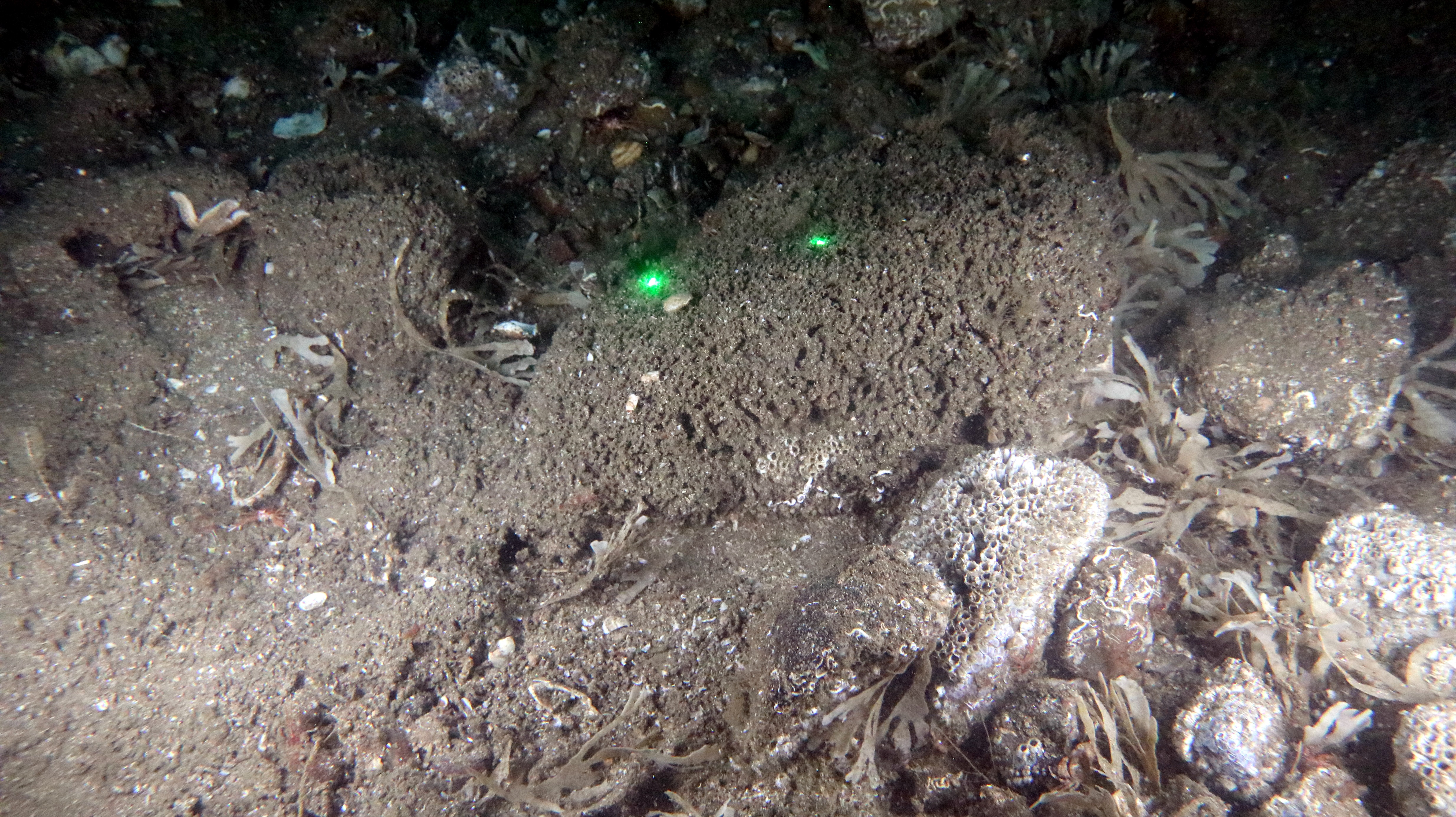
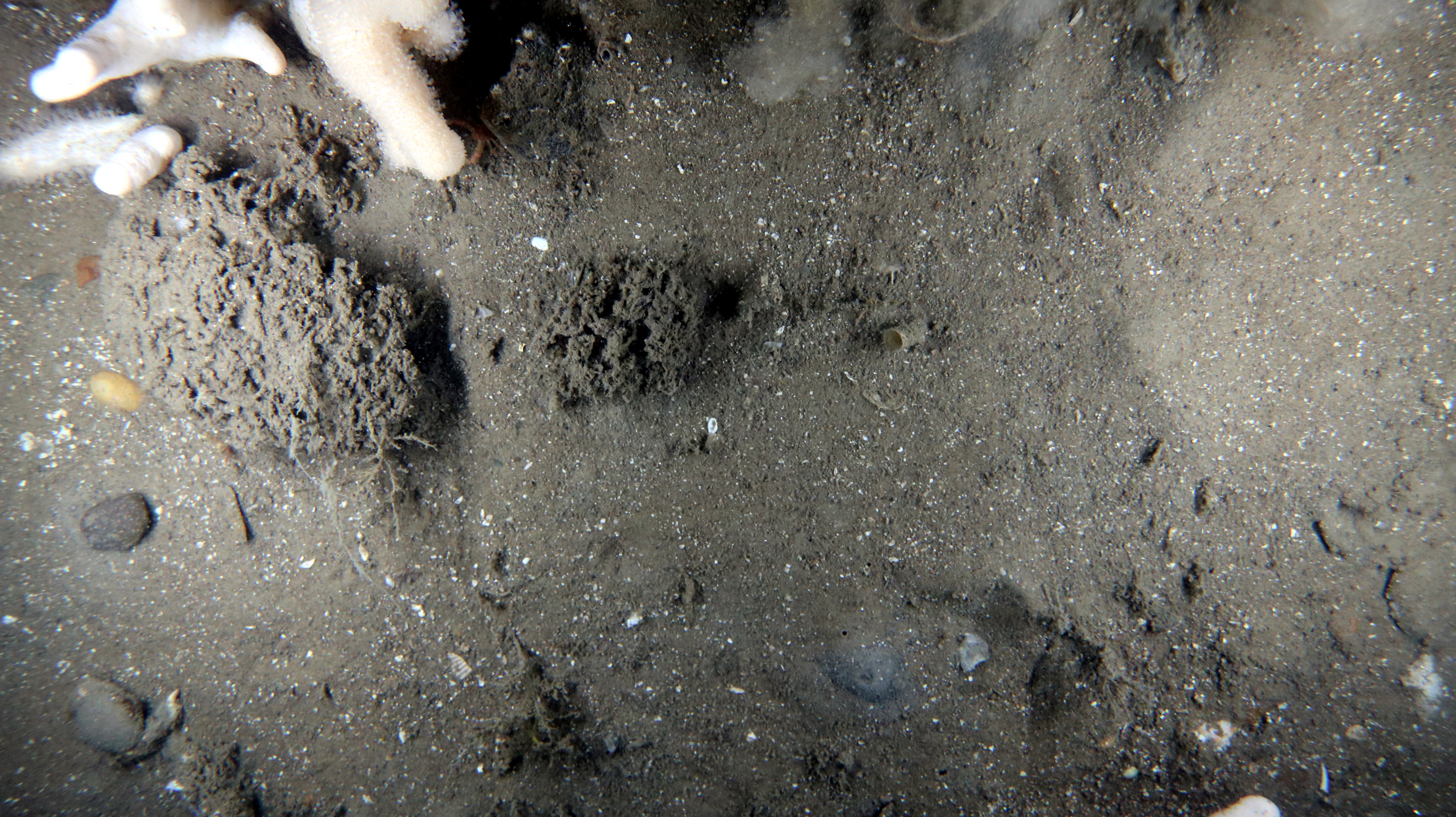
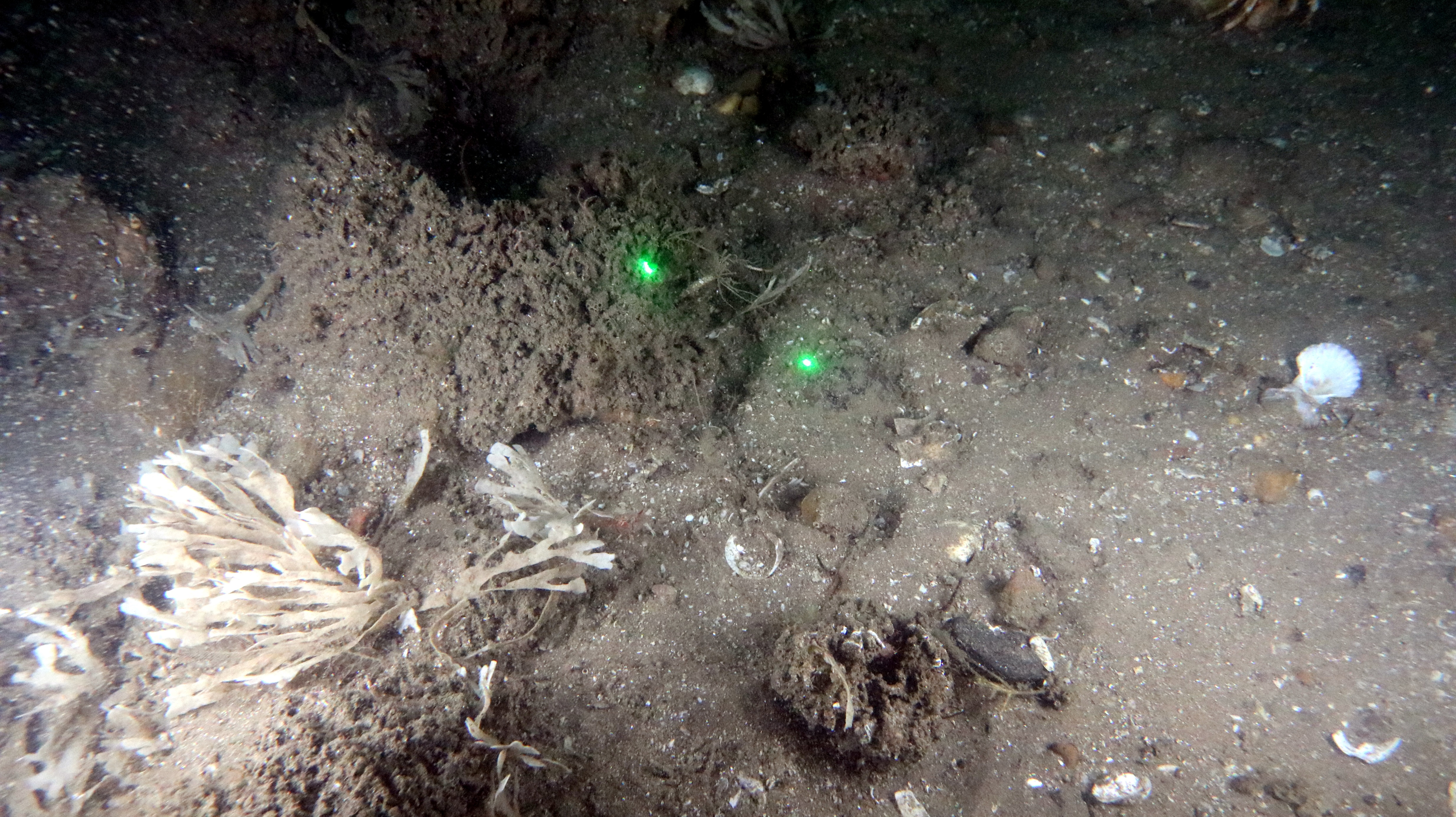
6.2.2. Annex 1 Stony Reef Assessment
Site | Sediment Description | Elevation (m) | Composition (% Cover) | Extent (m2) | Reef Definition | Reefiness | Sample Station Reefiness Assessment | Representative Image | ||
|---|---|---|---|---|---|---|---|---|---|---|
|
| Elevation | Composition | Extent | ||||||
ST101 | Moderate Energy Circalittoral Rock | 0.064-5 | 14.58 | <25 | Medium | Low | Not a Reef | Not a Reef | Not a Reef |
|
ST101 | Moderate Energy Circalittoral Rock | 0.064-5 | 40.57 | <25 | Medium | Medium | Not a Reef | Not a Reef | ||
ST107 | Moderate Energy Circalittoral Rock | 0.064-5 | 54.48 | >25 | Medium | Medium | Medium | Medium | Low |
|
ST107 | Moderate Energy Circalittoral Rock | 0.064-5 | 51.85 | >25 | Medium | Medium | Medium | Medium | ||
ST107 | Moderate Energy Circalittoral Rock | 0.064-5 | 24.46 | >25 | Medium | Low | Medium | Low | ||
ST107 | Moderate Energy Circalittoral Rock | 0.064-5 | 44.79 | >25 | Medium | Medium | Medium | Medium | ||
ST107 | Moderate Energy Circalittoral Rock | 0.064-5 | 30.86 | >25 | Medium | Low | Medium | Low | ||
ST107 | Moderate Energy Circalittoral Rock | 0.064-5 | 34.16 | >25 | Medium | Low | Medium | Low | ||
ST107 | Moderate Energy Circalittoral Rock | 0.064-5 | 9.56 | >25 | Medium | Not a Reef | Medium | Not a Reef | ||
ST107 | Moderate Energy Circalittoral Rock | 0.064-5 | 40.92 | >25 | Medium | Medium | Medium | Medium | ||
ST107 | Moderate Energy Circalittoral Rock | 0.064-5 | 36.18 | >25 | Medium | Low | Medium | Low | ||
ST107 | Moderate Energy Circalittoral Rock | 0.064-5 | 0.00 | >25 | Medium | Not a Reef | Medium | Not a Reef | ||
ST107 | Moderate Energy Circalittoral Rock | 0.064-5 | 45.70 | >25 | Medium | Medium | Medium | Medium | ||
ST107 | Moderate Energy Circalittoral Rock | 0.064-5 | 0.00 | >25 | Medium | Not a Reef | Medium | Not a Reef | ||
ST107 | Moderate Energy Circalittoral Rock | 0.064-5 | 31.05 | >25 | Medium | Low | Medium | Low | ||
ST107 | Moderate Energy Circalittoral Rock | 0.064-5 | 19.97 | >25 | Medium | Low | Medium | Low | ||
ST107 | Moderate Energy Circalittoral Rock | 0.064-5 | 38.32 | >25 | Medium | Low | Medium | Low | ||
ST107 | Moderate Energy Circalittoral Rock | 0.064-5 | 66.09 | >25 | Medium | Medium | Medium | Medium | ||
ST107 | Moderate Energy Circalittoral Rock | 0.064-5 | 25.63 | >25 | Medium | Low | Medium | Low | ||
ST107 | Moderate Energy Circalittoral Rock | 0.064-5 | 32.59 | >25 | Medium | Low | Medium | Low | ||
ST107 | Moderate Energy Circalittoral Rock | 0.064-5 | 30.47 | >25 | Medium | Low | Medium | Low | ||
ST107 | Moderate Energy Circalittoral Rock | 0.064-5 | 36.83 | >25 | Medium | Low | Medium | Low | ||
ST107 | Moderate Energy Circalittoral Rock | 0.064-5 | 27.40 | >25 | Medium | Low | Medium | Low | ||
ST107 | Moderate Energy Circalittoral Rock | 0.064-5 | 34.56 | >25 | Medium | Low | Medium | Low | ||
ST107 | Moderate Energy Circalittoral Rock | 0.064-5 | 31.60 | >25 | Medium | Low | Medium | Low | ||
ST107 | Moderate Energy Circalittoral Rock | 0.064-5 | 57.90 | >25 | Medium | Medium | Medium | Medium | ||
ST107 | Moderate Energy Circalittoral Rock | 0.064-5 | 50.56 | >25 | Medium | Medium | Medium | Medium | ||
ST107 | Moderate Energy Circalittoral Rock | 0.064-5 | 52.08 | >25 | Medium | Medium | Medium | Medium | ||
ST107 | Moderate Energy Circalittoral Rock | 0.064-5 | 30.88 | >25 | Medium | Low | Medium | Low | ||
ST107 | Moderate Energy Circalittoral Rock | 0.064-5 | 53.51 | >25 | Medium | Medium | Medium | Medium | ||
ST107 | Moderate Energy Circalittoral Rock | 0.064-5 | 66.54 | >25 | Medium | Medium | Medium | Medium | ||
ST107 | Moderate Energy Circalittoral Rock | 0.064-5 | 37.10 | >25 | Medium | Low | Medium | Low | ||
ST107 | Moderate Energy Circalittoral Rock | 0.064-5 | 45.88 | >25 | Medium | Medium | Medium | Medium | ||
ST110 | Moderate Energy Circalittoral Rock | 0.064-5 | 12.30 | >25 | Medium | Low | Medium | Low | Low |
|
ST110 | Moderate Energy Circalittoral Rock | 0.064-5 | 20.83 | >25 | Medium | Low | Medium | Low | ||
ST110 | Moderate Energy Circalittoral Rock | 0.064-5 | 36.96 | >25 | Medium | Low | Medium | Low | ||
ST110 | Moderate Energy Circalittoral Rock | 0.064-5 | 34.20 | >25 | Medium | Low | Medium | Low | ||
ST110 | Moderate Energy Circalittoral Rock | 0.064-5 | 10.79 | >25 | Medium | Low | Medium | Low | ||
ST110 | Moderate Energy Circalittoral Rock | 0.064-5 | 38.38 | >25 | Medium | Low | Medium | Low | ||
ST110 | Moderate Energy Circalittoral Rock | 0.064-5 | 62.21 | >25 | Medium | Medium | Medium | Medium | ||
ST110 | Moderate Energy Circalittoral Rock | 0.064-5 | 31.63 | >25 | Medium | Low | Medium | Low | ||
ST110 | Moderate Energy Circalittoral Rock | 0.064-5 | 44.95 | >25 | Medium | Low | Medium | Medium | ||
ST110 | Moderate Energy Circalittoral Rock | 0.064-5 | 52.75 | >25 | Medium | Medium | Medium | Medium | ||
ST110 | Moderate Energy Circalittoral Rock | < 0.064 | 10.86 | >25 | Low | Low | Medium | Low | ||
ST02 | Moderate Energy Circalittoral Rock | < 0.064 | 12.66 | <25 | Low | Low | Not a Reef | Not a Reef | Not a Reef |
|
ST02 | Moderate Energy Circalittoral Rock | < 0.064 | 17.57 | <25 | Low | Low | Not a Reef | Not a Reef | ||
ST20 | High Energy Circalittoral Rock | 0.064-5 | 22.31 | >25 | Medium | Low | Medium | Low | Low |
|
ST38 | Moderate Energy Circalittoral Rock | 0.064-5 | 10.18 | > 25 | Medium | Low | Medium | Low | Low |
|
ST38 | Moderate Energy Circalittoral Rock | 0.064-5 | 12.44 | > 25 | Medium | Low | Medium | Low | ||
ST38 | Moderate Energy Circalittoral Rock | 0.064-5 | 15.81 | > 25 | Medium | Low | Medium | Low | ||
ST38 | Moderate Energy Circalittoral Rock | 0.064-5 | 11.60 | > 25 | Medium | Low | Medium | Low | ||
ST38 | Moderate Energy Circalittoral Rock | < 0.064 | 6.35 | > 25 | Low | Not a Reef | Medium | Not a Reef | ||
ST04 | Moderate Energy Circalittoral Rock | 0.064-5 | 14.66 | < 25 | Medium | Low | Not a Reef | Not a Reef | Not a Reef |
|
ST04 | Moderate Energy Circalittoral Rock | 0.064-5 | 15.52 | < 25 | Medium | Low | Not a Reef | Not a Reef | ||
ST61 | Moderate Energy Circalittoral Rock | 0.064-5 | 46.91 | < 25 | Medium | Medium | Not a Reef | Not a Reef | Not a Reef |
|
ST69 | High Energy Circalittoral Rock | < 0.064 | 10.86 | < 25 | Low | Low | Not a Reef | Not a Reef | Not a Reef |
|
ST69 | High Energy Circalittoral Rock | < 0.064 | 11.92 | < 25 | Low | Low | Not a Reef | Not a Reef | ||
ST69 | High Energy Circalittoral Rock | < 0.064 | 11.99 | < 25 | Low | Low | Not a Reef | Not a Reef | ||
ST69 | High Energy Circalittoral Rock | < 0.064 | 18.24 | < 25 | Low | Low | Not a Reef | Not a Reef | ||
ST69 | High Energy Circalittoral Rock | < 0.064 | 11.17 | < 25 | Low | Low | Not a Reef | Not a Reef | ||
ST69 | High Energy Circalittoral Rock | < 0.064 | 13.56 | < 25 | Low | Low | Not a Reef | Not a Reef | ||
ST83 | Moderate Energy Circalittoral Rock | 0.064-5 | 26.02 | < 25 | Medium | Low | Not a Reef | Not a Reef | Not a Reef |
|
ST84 | Moderate Energy Circalittoral Rock | 0.064-5 | 22.63 | < 25 | Medium | Low | Not a Reef | Not a Reef | Not a Reef |
|
ST84 | Moderate Energy Circalittoral Rock | < 0.064 | 9.31 | < 25 | Low | Not a Reef | Not a Reef | Not a Reef | ||
ST84 | Moderate Energy Circalittoral Rock | 0.064-5 | 25.13 | < 25 | Medium | Low | Not a Reef | Not a Reef | ||
ST89 | Moderate Energy Circalittoral Rock | 0.064-5 | 76.33 | >25 | Medium | Medium | Medium | Medium | Medium |
|
ST89 | Moderate Energy Circalittoral Rock | 0.064-5 | 49.53 | >25 | Medium | Medium | Medium | Medium | ||
ST89 | Moderate Energy Circalittoral Rock | 0.064-5 | 82.78 | >25 | Medium | Medium | Medium | Medium | ||
ST89 | Moderate Energy Circalittoral Rock | 0.064-5 | 62.29 | >25 | Medium | Medium | Medium | Medium | ||
ST89 | Moderate Energy Circalittoral Rock | 0.064-5 | 40.52 | >25 | Medium | Medium | Medium | Medium | ||
ST89 | Moderate Energy Circalittoral Rock | 0.064-5 | 54.55 | >25 | Medium | Medium | Medium | Medium | ||
ST89 | Moderate Energy Circalittoral Rock | 0.064-5 | 73.25 | >25 | Medium | Medium | Medium | Medium | ||
ST89 | Moderate Energy Circalittoral Rock | 0.064-5 | 74.03 | >25 | Medium | Medium | Medium | Medium | ||
ST89 | Moderate Energy Circalittoral Rock | 0.064-5 | 33.98 | >25 | Medium | Low | Medium | Low | ||
ST89 | Moderate Energy Circalittoral Rock | 0.064-5 | 41.45 | >25 | Medium | Medium | Medium | Medium | ||
ST89 | Moderate Energy Circalittoral Rock | 0.064-5 | 51.84 | >25 | Medium | Medium | Medium | Medium | ||
ST89 | Moderate Energy Circalittoral Rock | 0.064-5 | 85.23 | >25 | Medium | Medium | Medium | Medium | ||
ST89 | Moderate Energy Circalittoral Rock | 0.064-5 | 54.81 | >25 | Medium | Medium | Medium | Medium | ||
ST89 | Moderate Energy Circalittoral Rock | 0.064-5 | 58.93 | >25 | Medium | Medium | Medium | Medium | ||
ST89 | Moderate Energy Circalittoral Rock | 0.064-5 | 65.79 | >25 | Medium | Medium | Medium | Medium | ||
ST89 | Moderate Energy Circalittoral Rock | 0.064-5 | 38.39 | >25 | Medium | Medium | Medium | Low | ||
ST89 | Moderate Energy Circalittoral Rock | 0.064-5 | 68.00 | >25 | Medium | Medium | Medium | Medium | ||
ST89 | Moderate Energy Circalittoral Rock | 0.064-5 | 67.62 | >25 | Medium | Medium | Medium | Medium | ||
ST89 | Moderate Energy Circalittoral Rock | 0.064-5 | 36.92 | >25 | Medium | Low | Medium | Low | ||
ST89 | Moderate Energy Circalittoral Rock | 0.064-5 | 39.00 | >25 | Medium | Low | Medium | Low | ||
ST89 | Moderate Energy Circalittoral Rock | 0.064-5 | 41.97 | >25 | Medium | Medium | Medium | Medium | ||
ST89 | Moderate Energy Circalittoral Rock | 0.064-5 | 72.92 | >25 | Medium | Medium | Medium | Medium | ||
ST89 | Moderate Energy Circalittoral Rock | 0.064-5 | 52.35 | >25 | Medium | Medium | Medium | Medium | ||
ST89 | Moderate Energy Circalittoral Rock | 0.064-5 | 95.25 | >25 | Medium | High | Medium | Medium | ||
ST89 | Moderate Energy Circalittoral Rock | 0.064-5 | 30.15 | >25 | Medium | Low | Medium | Low | ||
ST89 | Moderate Energy Circalittoral Rock | < 0.064 | 15.79 | >25 | Low | Low | Medium | Low | ||
ST89 | Moderate Energy Circalittoral Rock | < 0.064 | 30.07 | >25 | Low | Low | Medium | Low | ||
ST89 | Moderate Energy Circalittoral Rock | < 0.064 | 2.45 | >25 | Low | Not a Reef | Medium | Not a Reef | ||
ST89 | Moderate Energy Circalittoral Rock | < 0.064 | 16.06 | >25 | Low | Low | Medium | Low | ||
ST89 | Moderate Energy Circalittoral Rock | < 0.064 | 17.21 | >25 | Low | Low | Medium | Low | ||
ST89 | Moderate Energy Circalittoral Rock | < 0.064 | 20.23 | >25 | Low | Low | Medium | Low | ||
ST89 | Moderate Energy Circalittoral Rock | < 0.064 | 14.72 | >25 | Low | Low | Medium | Low | ||
ST89 | Moderate Energy Circalittoral Rock | < 0.064 | 20.61 | >25 | Low | Low | Medium | Low | ||
ST89 | Moderate Energy Circalittoral Rock | < 0.064 | 0.00 | >25 | Low | Not a Reef | Medium | Not a Reef | ||
ST89 | Subtidal Coarse Sediment | < 0.064 | 5.78 | >25 | Low | Not a Reef | Medium | Not a Reef | ||
ST89 | Moderate Energy Circalittoral Rock | < 0.064 | 5.78 | >25 | Low | Not a Reef | Medium | Not a Reef | ||
ST89 | Moderate Energy Circalittoral Rock | < 0.064 | 5.78 | >25 | Low | Not a Reef | Medium | Not a Reef | ||
ST89 | Subtidal Coarse Sediment | < 0.064 | 5.78 | >25 | Low | Not a Reef | Medium | Not a Reef | ||
ST89 | Moderate Energy Circalittoral Rock | < 0.064 | 11.24 | >25 | Low | Low | Medium | Low | ||
ST111 | High Energy Infralittoral Rock |
| 35.82 | >25 |
| Low | Medium | Low | Medium |
|
ST111 | High Energy Infralittoral Rock |
| 99.31 | >25 |
| High | Medium | Medium | ||
ST111 | Moderate Energy Circalittoral Rock |
| 98.21 | >25 |
| High | Medium | Medium | ||
ST111 | Moderate Energy Circalittoral Rock |
| 99.24 | >25 |
| High | Medium | Medium | ||
ST111 | Moderate Energy Circalittoral Rock |
| 99.54 | >25 |
| High | Medium | Medium | ||
ST111 | Moderate Energy Circalittoral Rock |
| 98.80 | >25 |
| High | Medium | Medium | ||
ST111 | Moderate Energy Circalittoral Rock |
| 37.19 | >25 |
| Low | Medium | Low | ||
ST111 | Moderate Energy Circalittoral Rock |
| 55.74 | >25 |
| Medium | Medium | Medium | ||
ST111 | Moderate Energy Circalittoral Rock |
| 99.92 | >25 |
| High | Medium | Medium | ||
ST111 | Moderate Energy Circalittoral Rock |
| 99.97 | >25 |
| High | Medium | Medium | ||
ST111 | Moderate Energy Circalittoral Rock |
| 42.67 | >25 |
| Medium | Medium | Medium | ||
ST111 | Moderate Energy Circalittoral Rock |
| 91.30 | >25 |
| Medium | Medium | Medium | ||
ST111 | Moderate Energy Circalittoral Rock |
| 98.92 | >25 |
| High | Medium | Medium | ||
ST111 | Moderate Energy Circalittoral Rock |
| 97.44 | >25 |
| High | Medium | Medium | ||
ST111 | Moderate Energy Circalittoral Rock |
| 98.72 | >25 |
| High | Medium | Medium | ||
ST111 | High Energy Infralittoral Rock |
| 99.98 | >25 |
| High | Medium | Medium | ||
ST111 | High Energy Infralittoral Rock |
| 99.97 | >25 |
| High | Medium | Medium | ||
ST111 | High Energy Infralittoral Rock |
| 88.43 | >25 |
| Medium | Medium | Medium | ||
ST111 | Moderate Energy Circalittoral Rock |
| 99.97 | >25 |
| High | Medium | Medium | ||
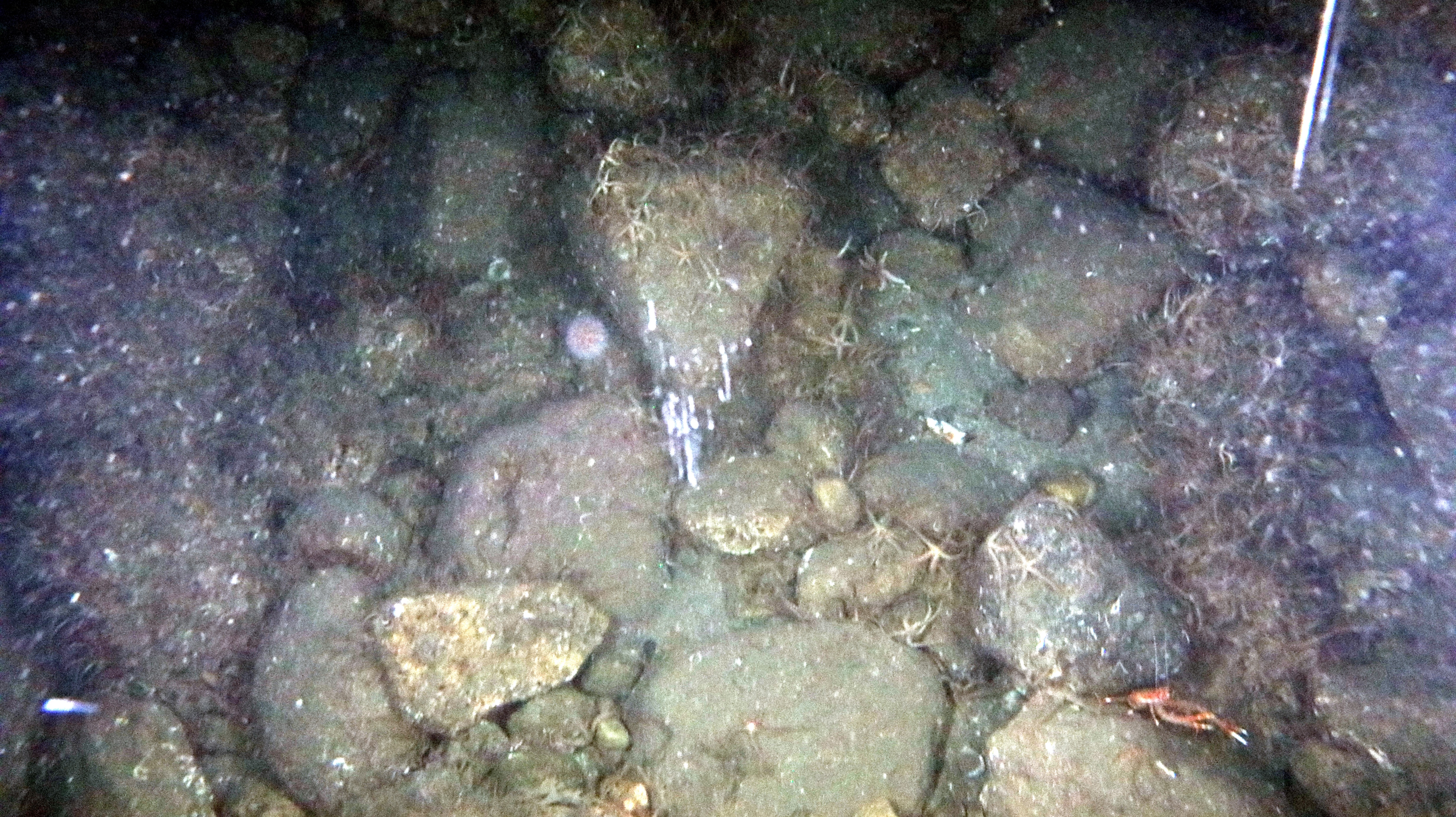
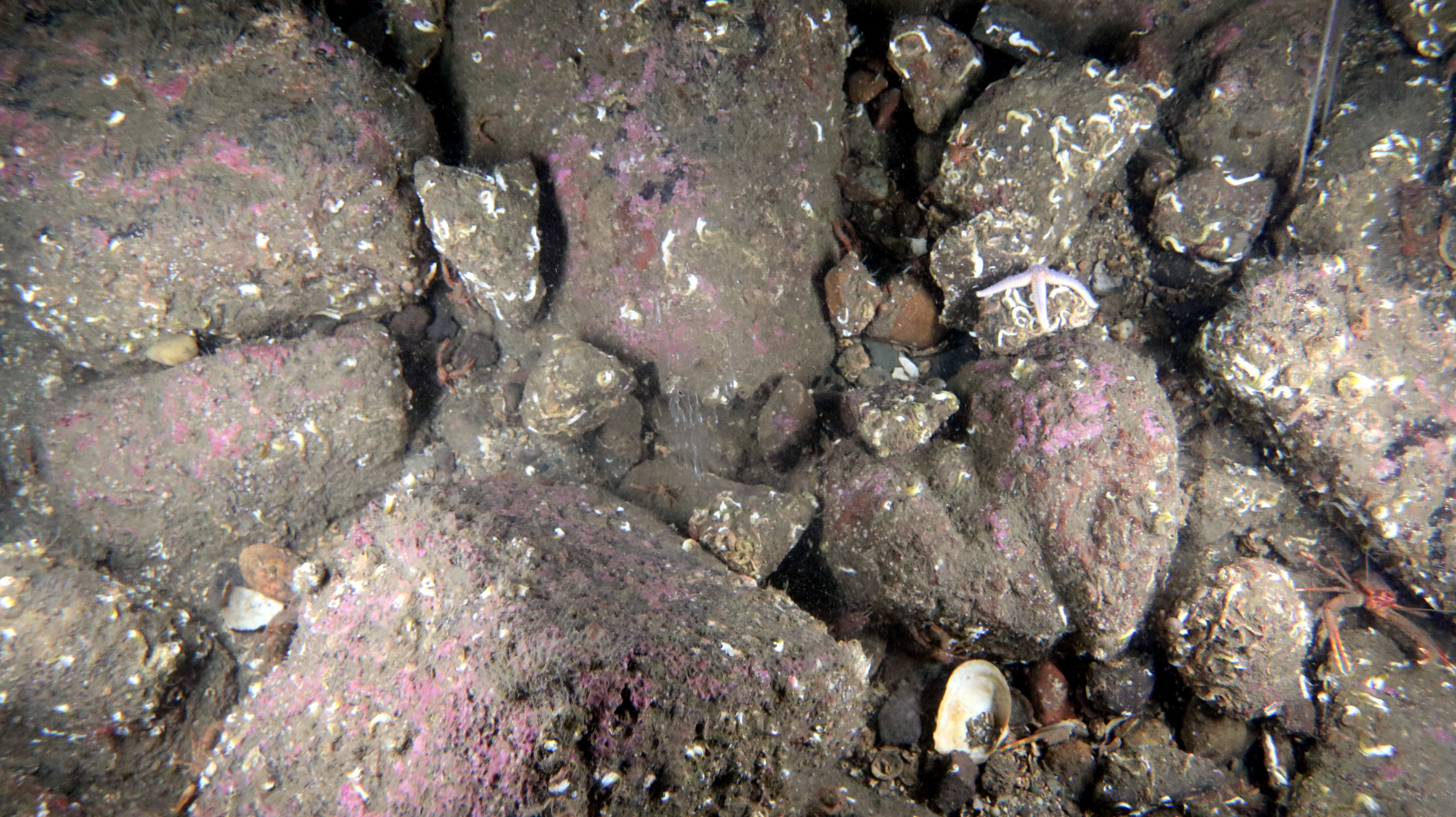
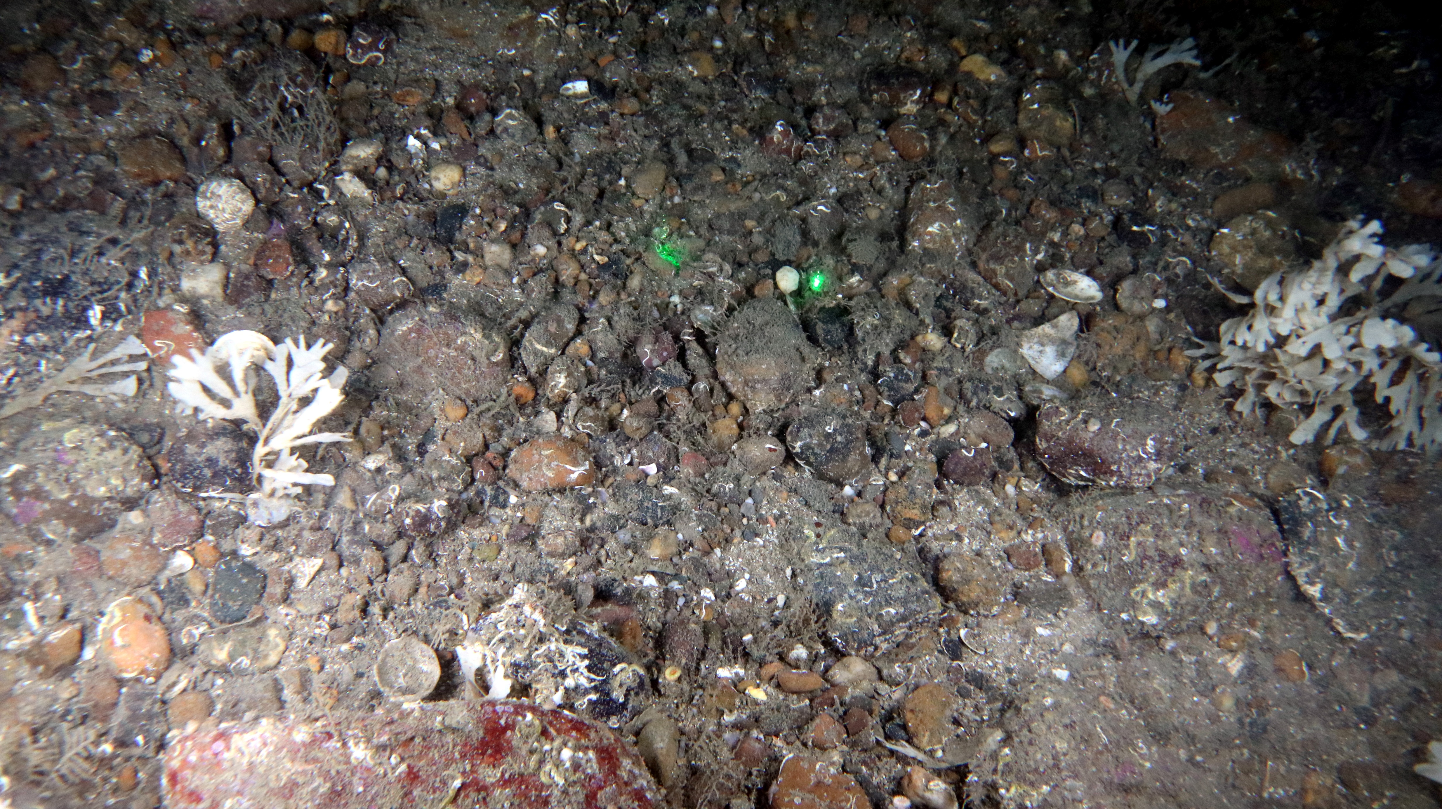
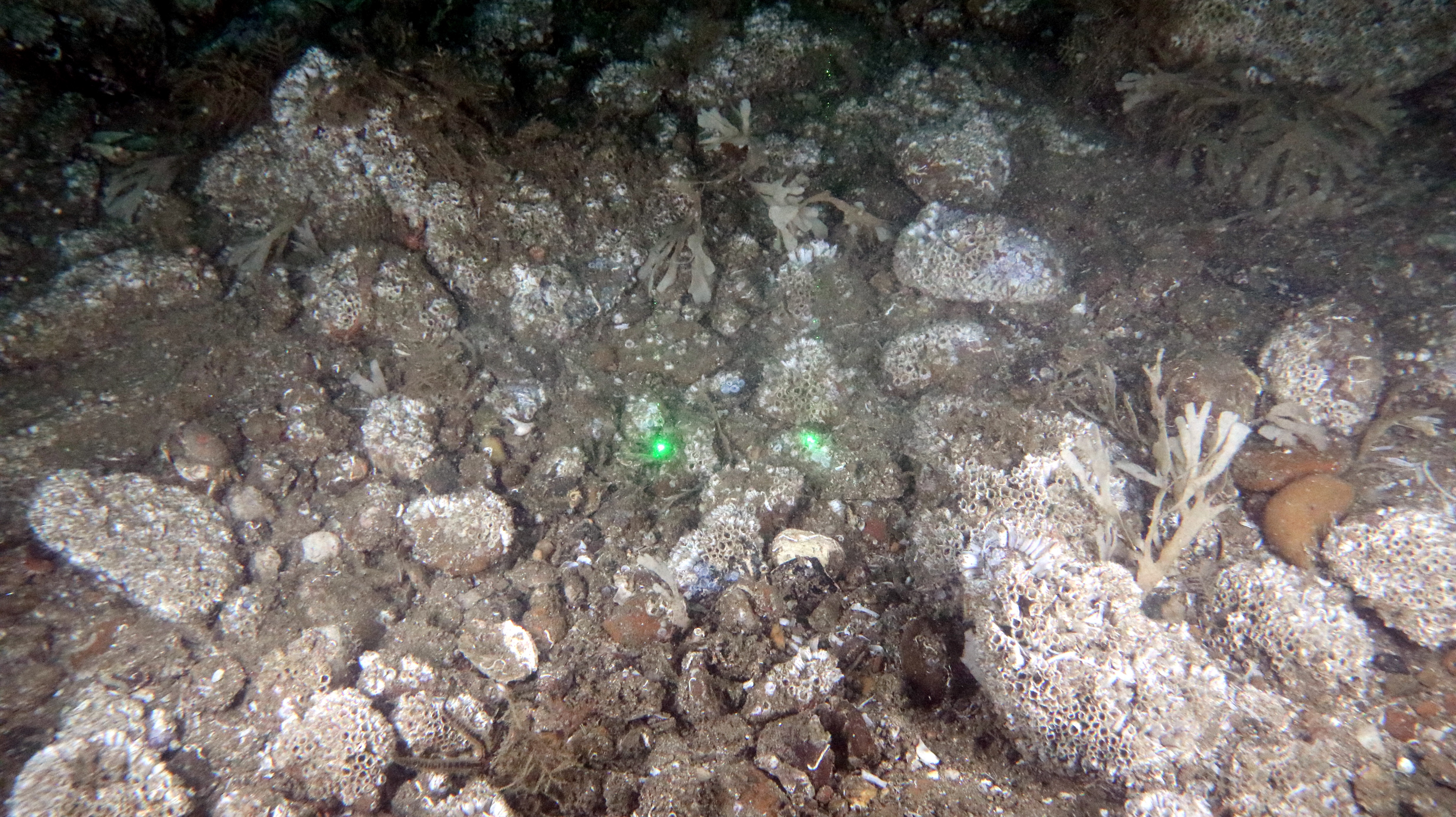
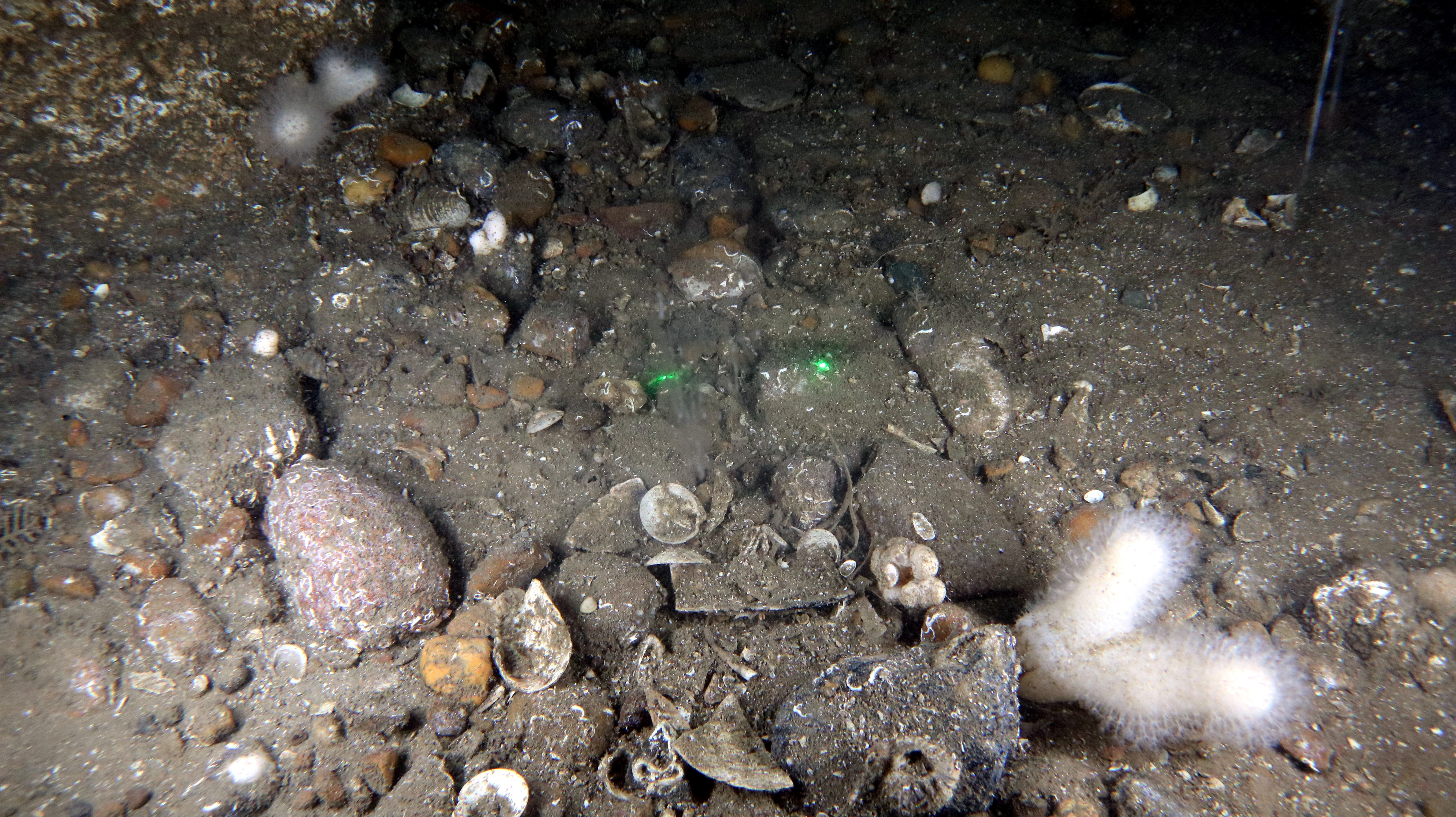
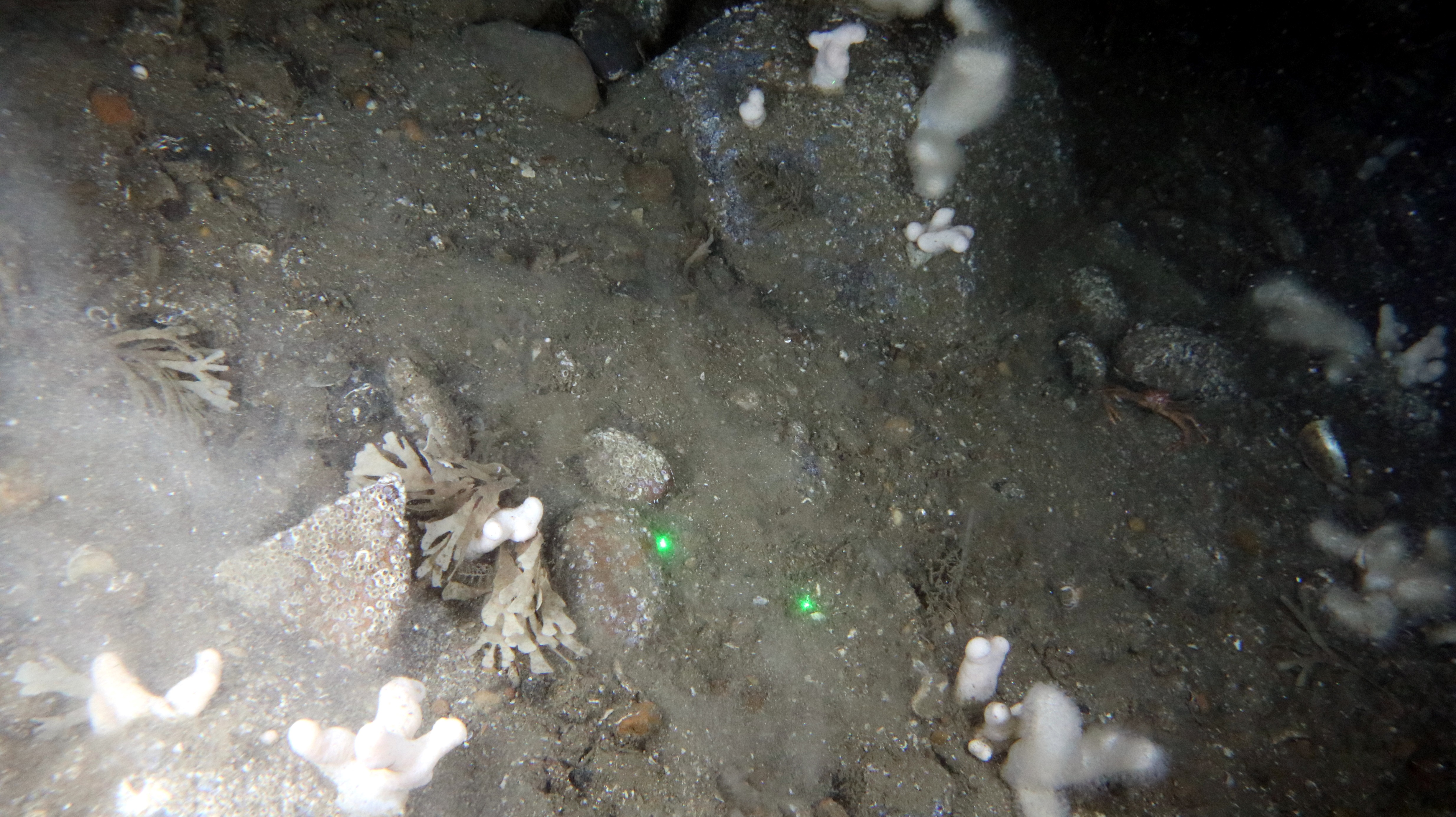
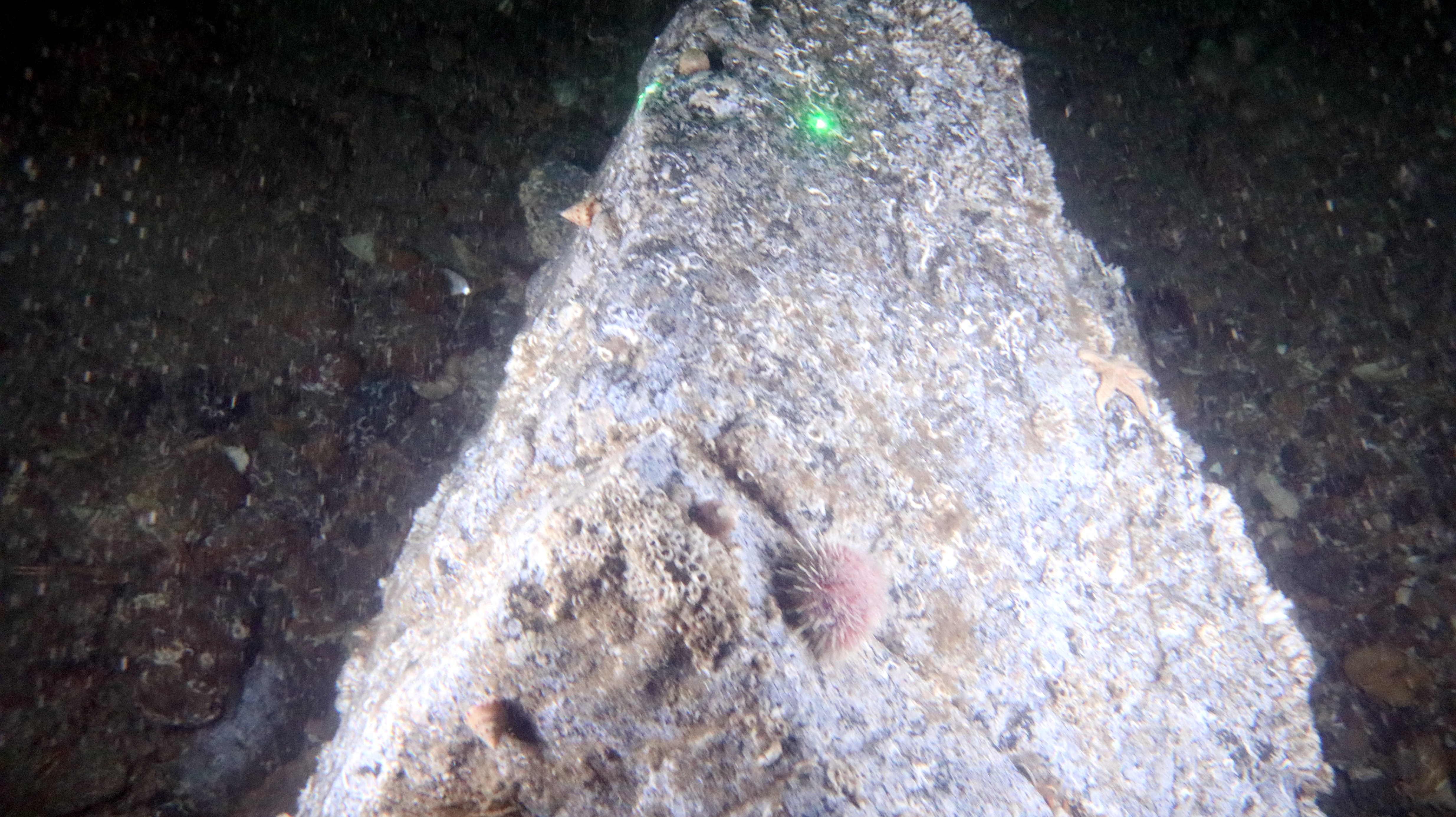
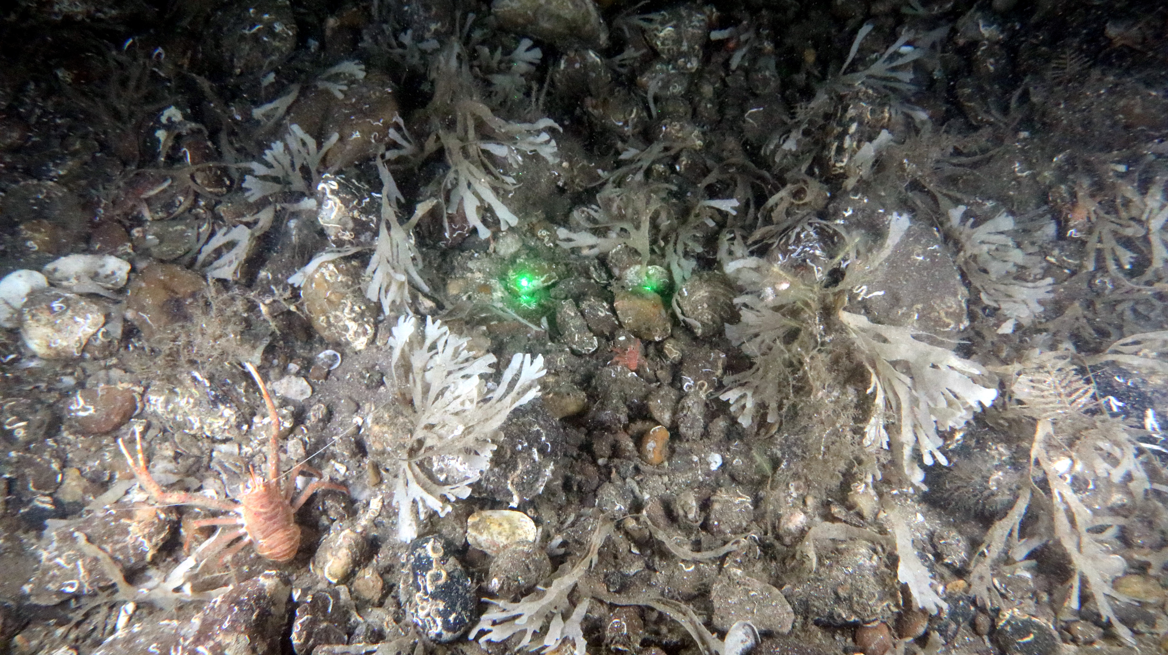
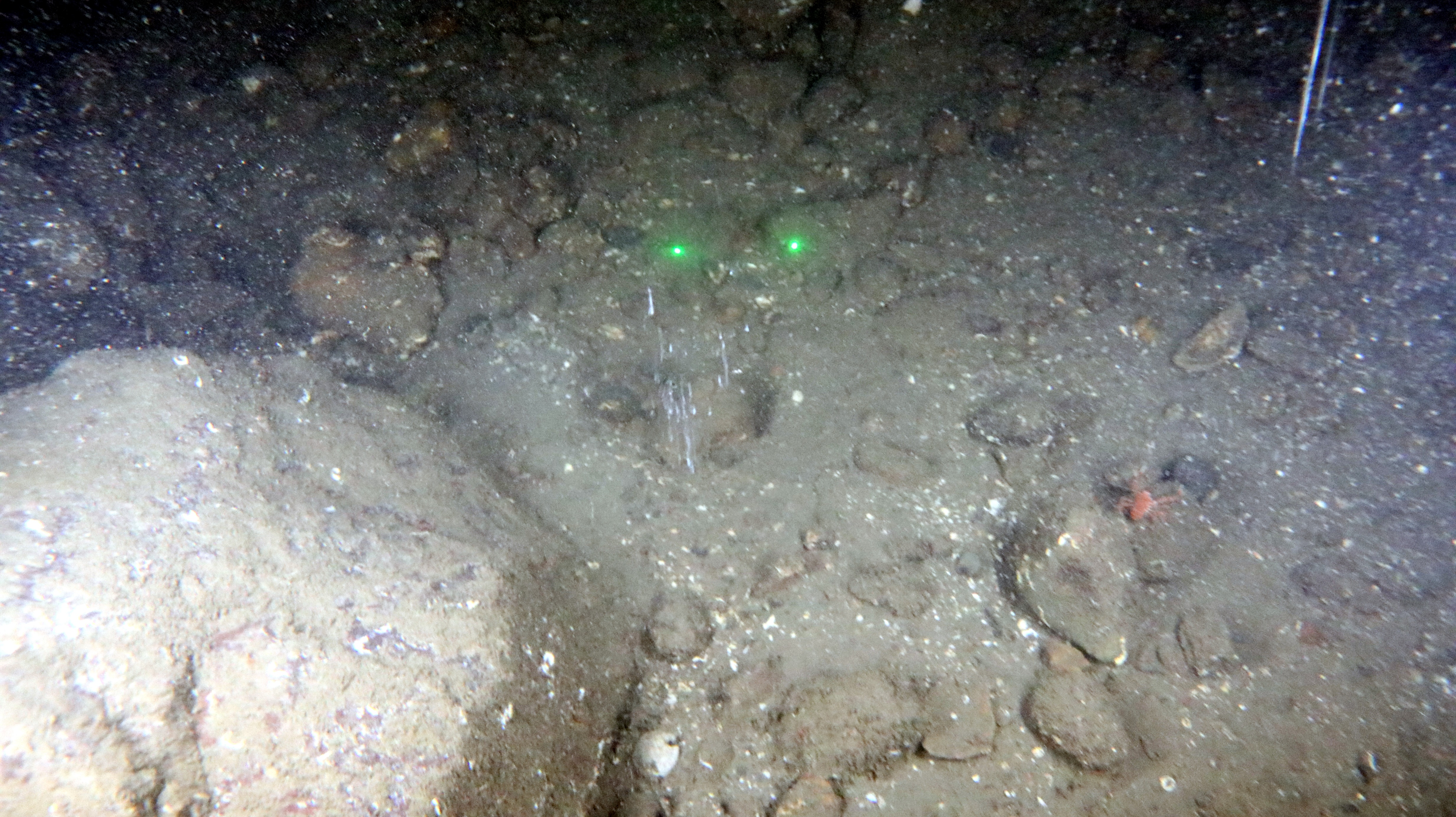
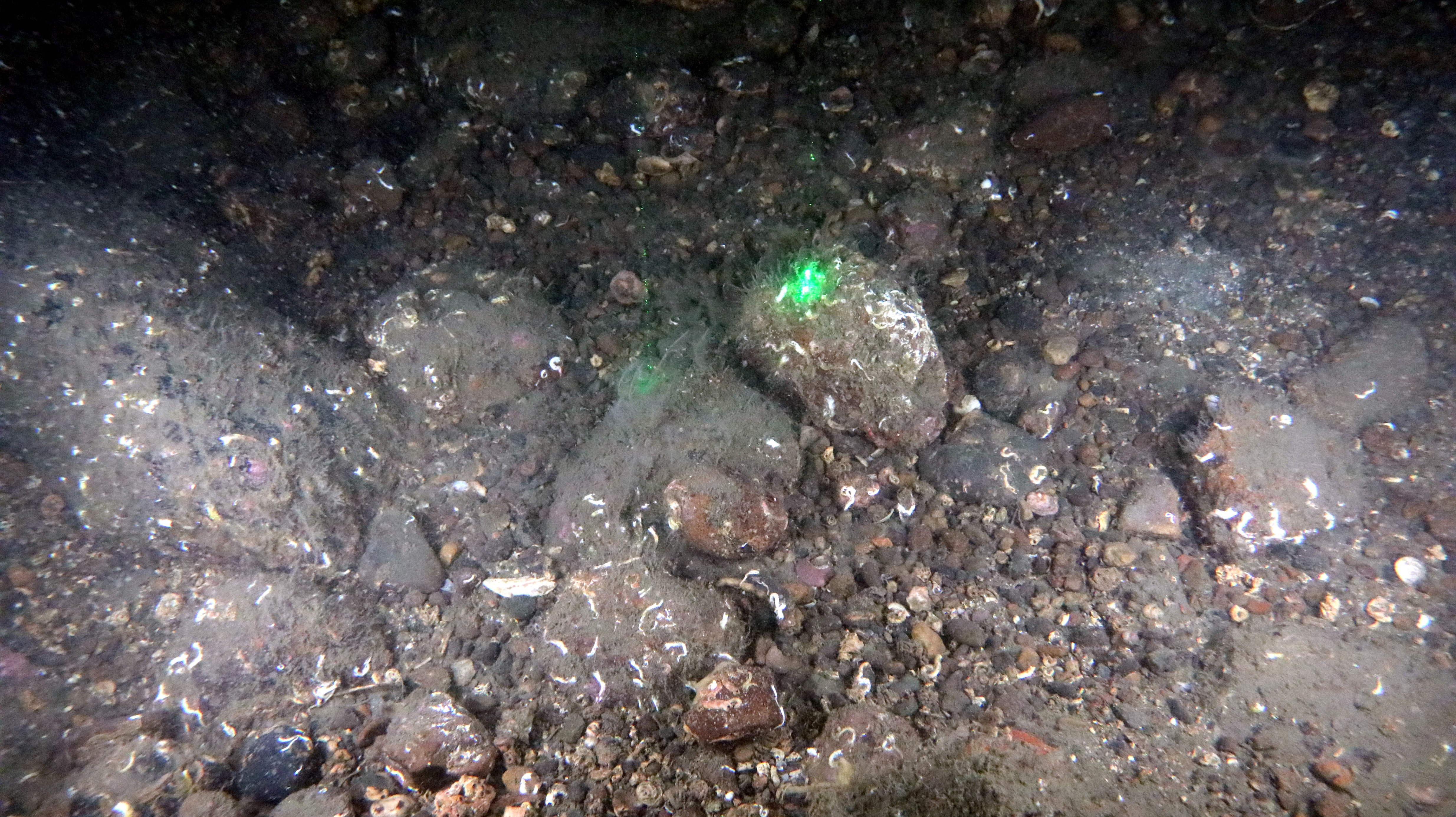
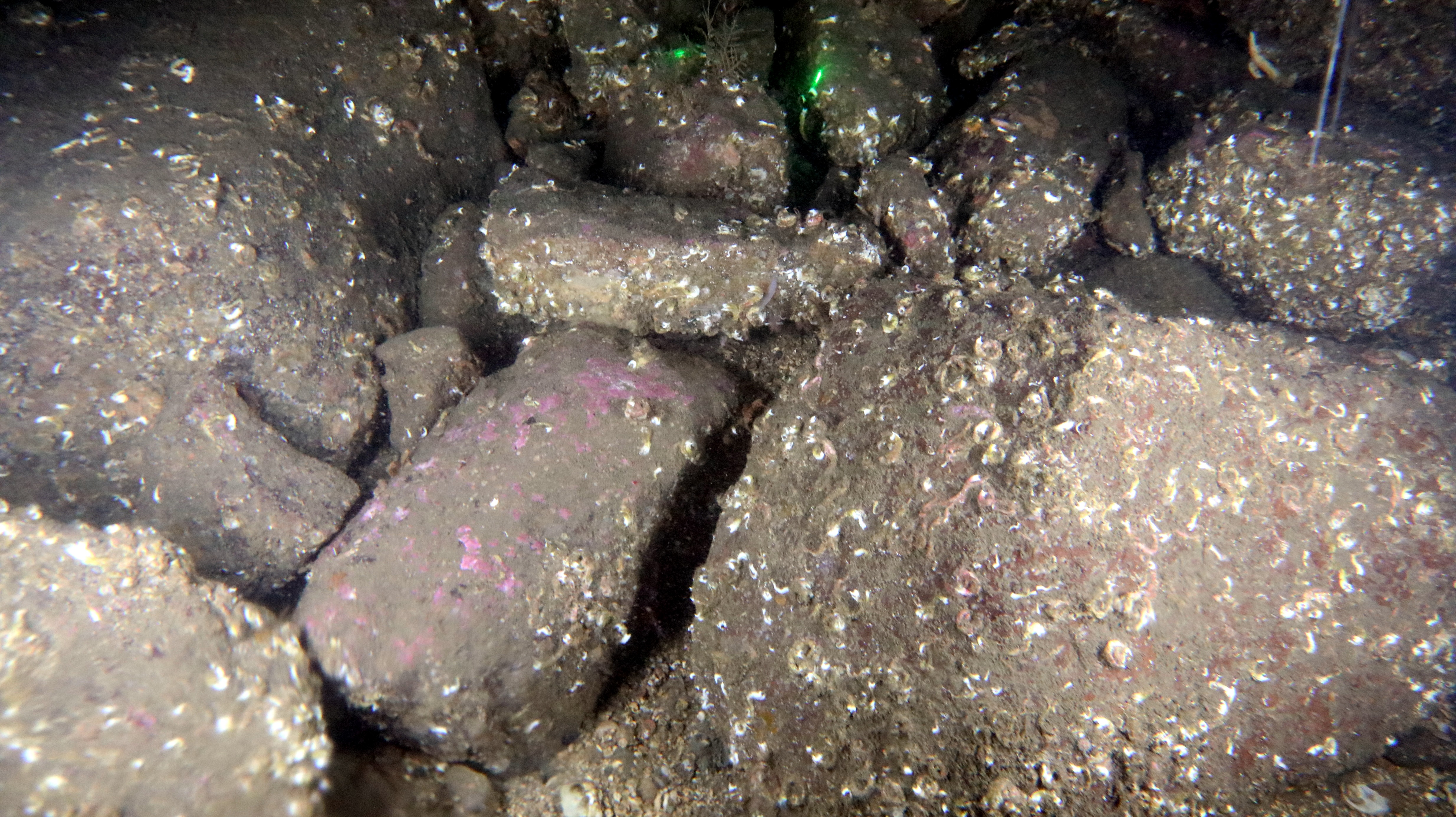
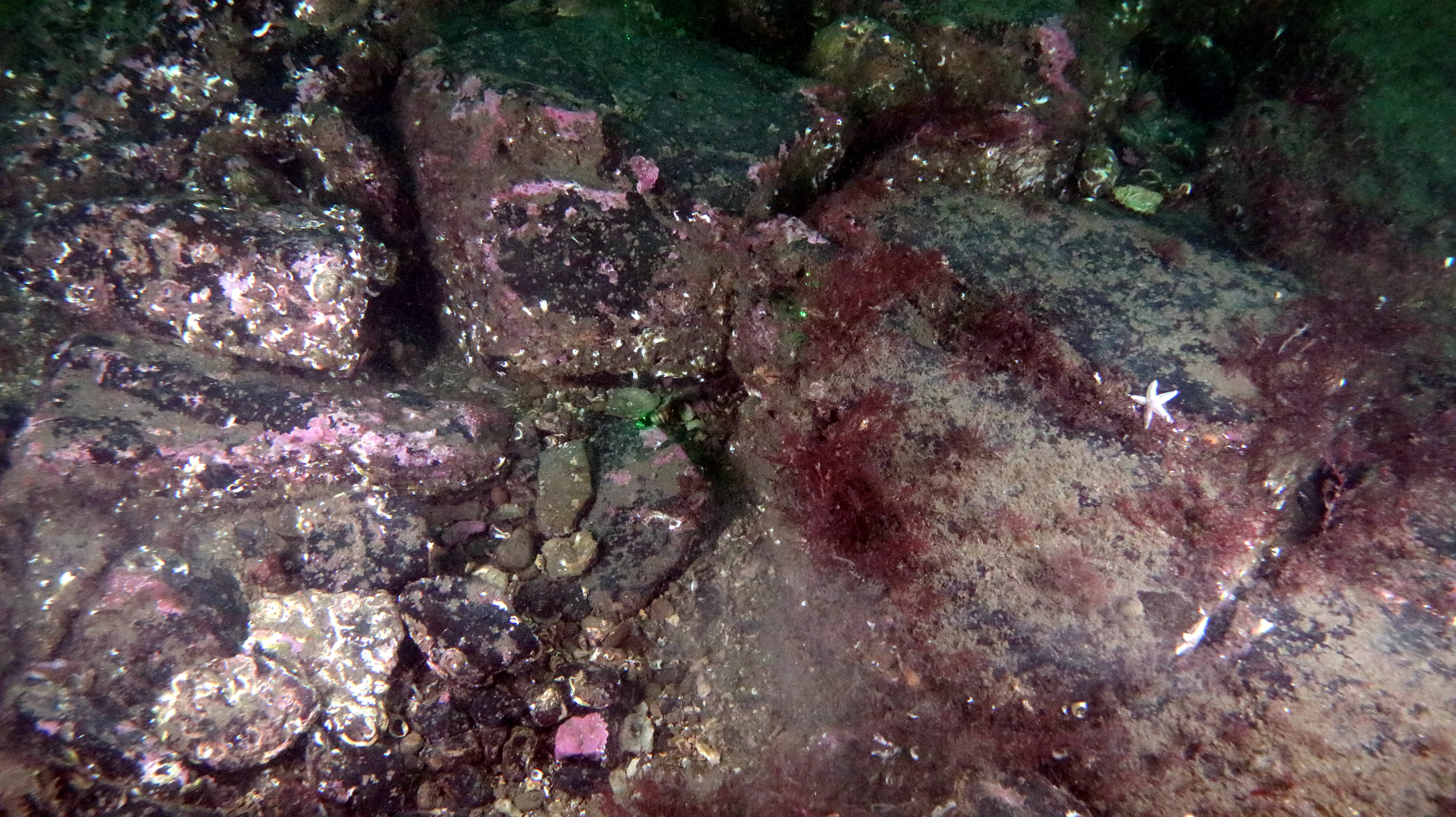
6.3. Annex C: Benthic Infaunal Data Multivariate Analysis Results
6.3. Annex C: Benthic Infaunal Data Multivariate Analysis Results

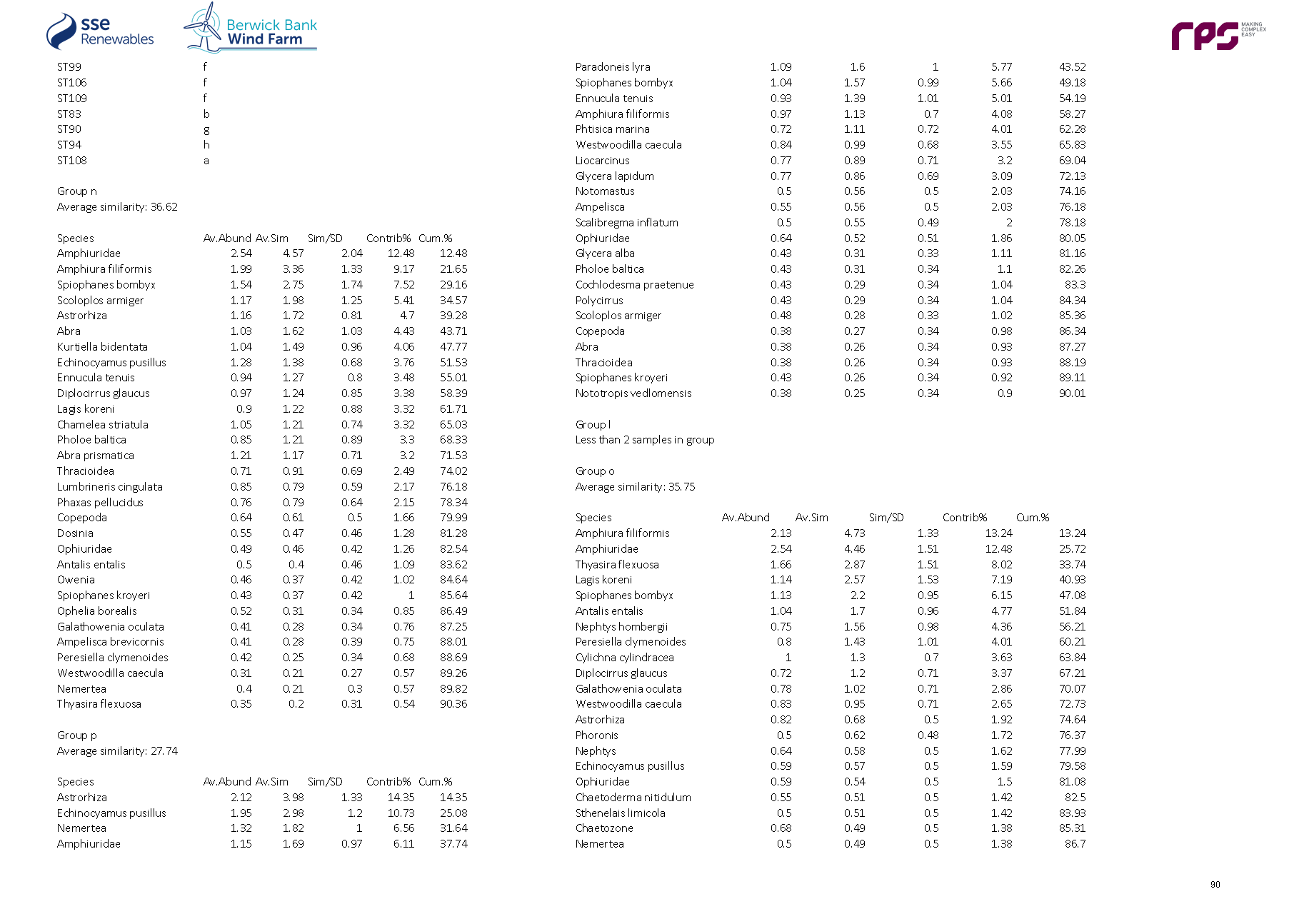
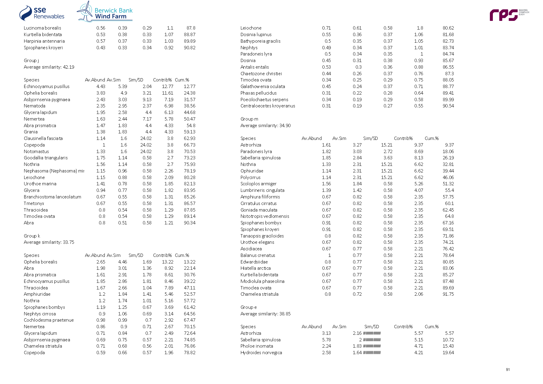
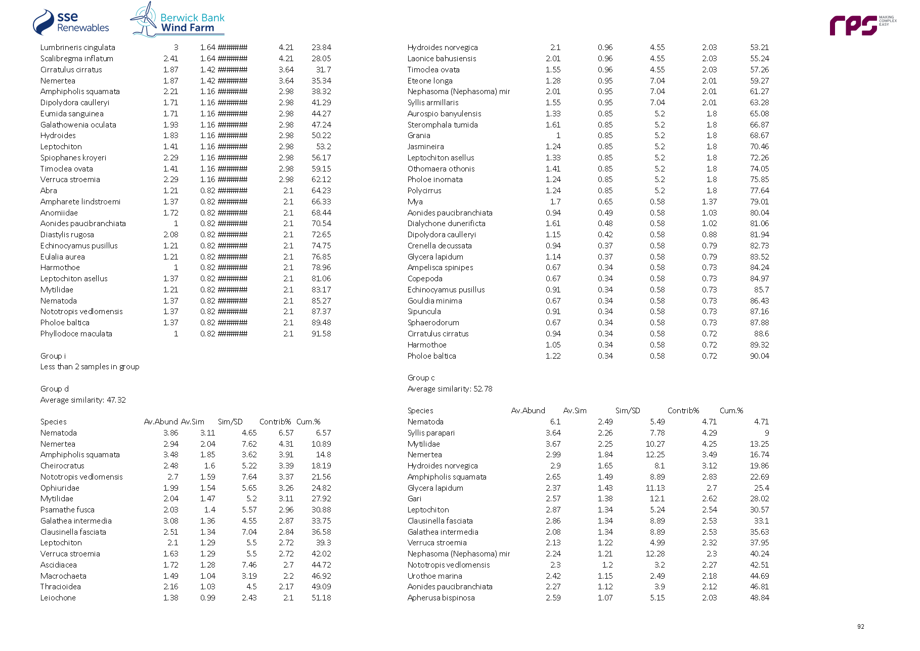
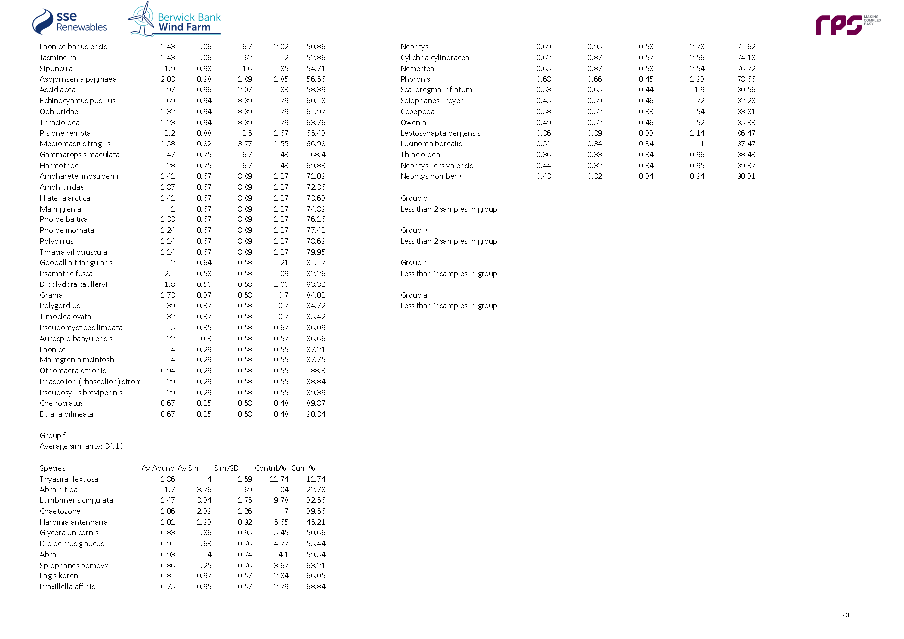
6.4. Annex D: Benthic Infaunal Data Univariate Analysis Results
6.4. Annex D: Benthic Infaunal Data Univariate Analysis Results
- S = number of species; N = abundance; B = Biomass (ash free dry mass in grams); d = Margalef’s index of Richness; J’ = Pielou’s Evenness index; H’ = Shannon-Wiener Diversity index; = Simpson’s Dominance index.
Sample Station | Preliminary Infaunal Biotope | S | N | Biomass (g) | d | J’ | H’ | |
|---|---|---|---|---|---|---|---|---|
3 | SS.SMu.CSaMu.AfilMysAnit | 38 | 51.34462 | 2.0122 | 9.394296 | 0.974647 | 3.545364 | 0.927258 |
5 | SS.SSa.Osa [Echinocyamus pusillus] | 26 | 35.04767 | 2.5463 | 7.028969 | 0.95703 | 3.118096 | 0.786332 |
6 | SS.SMu.CSaMu.AfilMysAnit | 32 | 45.99503 | 1.1123 | 8.097095 | 0.9696 | 3.360378 | 0.907029 |
7 | SS.SSa.OSa | 11 | 13.4641 | 0.2391 | 3.846114 | 0.982419 | 2.355737 | 0.87037 |
8 | SS.SMu.CSaMu.AfilMysAnit | 27 | 36.39109 | 1.3781 | 7.233627 | 0.976717 | 3.219099 | 0.9239 |
9 | SS.SMu.CSaMu.AfilMysAnit | 22 | 24.97469 | 0.2346 | 6.52607 | 0.991699 | 3.065384 | 0.94 |
10 | SS.SMu.CSaMu.AfilMysAnit | 31 | 37.21733 | 3.9247 | 8.294683 | 0.990233 | 3.400448 | 0.955729 |
11 | SS.SSa.OSa | 21 | 26.19151 | 0.9898 | 6.124758 | 0.981365 | 2.987788 | 0.917458 |
12 | SS.SMu.CSaMu.AfilNten | 18 | 22.66025 | 0.3696 | 5.447649 | 0.981703 | 2.837488 | 0.908203 |
13 | SS.SMu.CSaMu.AfilMysAnit | 27 | 34.80651 | 1.8878 | 7.324347 | 0.979834 | 3.229374 | 0.928254 |
14 | SS.SMu.CSaMu.AfilMysAnit | 33 | 44.50825 | 0.577 | 8.430649 | 0.977004 | 3.416101 | 0.929398 |
15 | SS.SSa.CFiSa.EpusOborApri | 39 | 56.43596 | 5.4517 | 9.422017 | 0.965479 | 3.537092 | 0.88759 |
16 | SS.SMu.CSaMu.AfilMysAnit | 29 | 38.63155 | 4.1692 | 7.66269 | 0.976877 | 3.289435 | 0.906868 |
17 | SS.SSa.CFiSa.EpusOborApri | 45 | 64.45246 | 4.7528 | 10.56187 | 0.965604 | 3.675728 | 0.912195 |
18 | SS.SSa.CFiSa.EpusOborApri | 31 | 44.18516 | 4.3805 | 7.918933 | 0.980778 | 3.367978 | 0.947531 |
19 | SS.SMu.CSaMu.AfilMysAnit | 33 | 40.64151 | 5.404 | 8.637467 | 0.989938 | 3.461326 | 0.95679 |
21 | SS.SMx.CMx.MysThyMx | 26 | 38.43353 | 2.5655 | 6.851323 | 0.971647 | 3.165719 | 0.899592 |
22 | SS.SMu.CSaMu.AfilMysAnit | 31 | 38.92407 | 1.4494 | 8.193111 | 0.986892 | 3.388973 | 0.947188 |
23 | SS.SMx.OMx.PoVen | 37 | 48.90884 | 1.1616 | 9.254598 | 0.986272 | 3.561348 | 0.955633 |
24 | SS.SMu.CSaMu.AfilMysAnit | 26 | 36.37356 | 7.604 | 6.956343 | 0.983286 | 3.203641 | 0.93875 |
26 | SS.SSa.CFiSa.EpusOborApri | 45 | 66.46548 | 182.2472 | 10.48447 | 0.972044 | 3.700242 | 0.942248 |
27 | SS.SSa.CFiSa.EpusOborApri | 33 | 39.02337 | 6.0886 | 8.733242 | 0.983923 | 3.440295 | 0.931292 |
28 | SS.SSa.CFiSa.EpusOborApri | 19 | 26.78084 | 1.4872 | 5.474974 | 0.97042 | 2.857342 | 0.869565 |
29 | SS.SSa.CFiSa.EpusOborApri | 16 | 27.46585 | 3.4235 | 4.527696 | 0.970507 | 2.690817 | 0.900496 |
30 | SS.SSa.CFiSa.EpusOborApri | 39 | 53.95271 | 2.5289 | 9.528328 | 0.969128 | 3.550462 | 0.920395 |
31 | SS.SSa.CFiSa.EpusOborApri | 37 | 53.90622 | 2.0032 | 9.028789 | 0.971357 | 3.507492 | 0.928885 |
32 | SS.SSa.CFiSa.EpusOborApri | 60 | 97.61815 | 2.0375 | 12.87911 | 0.974592 | 3.990317 | 0.964963 |
33 | SS.SSa.OSa | 21 | 25.12096 | 0.1068 | 6.204047 | 0.982705 | 2.991869 | 0.908304 |
34 | SS.SMu.CSaMu.AfilNten | 27 | 38.3543 | 2.4715 | 7.129408 | 0.959866 | 3.163563 | 0.887971 |
35 | SS.SMu.CSaMu.AfilMysAnit | 30 | 41.38426 | 2.0565 | 7.789625 | 0.965643 | 3.284341 | 0.866343 |
36 | SS.SBR.PoR.SspiMx | 84 | 139.8801 | 21.0183 | 16.79895 | 0.967588 | 4.287205 | 0.923138 |
37 | SS.SMu.CSaMu.AfilMysAnit | 33 | 41.90368 | 1.988 | 8.566747 | 0.983 | 3.437068 | 0.939532 |
40 | SS.SMu.CSaMu.AfilMysAnit | 20 | 25.90289 | 0.449 | 5.838331 | 0.984703 | 2.949908 | 0.923302 |
41 | SS.SMu.CSaMu.AfilMysAnit | 43 | 62.56973 | 3.4603 | 10.15405 | 0.976003 | 3.670942 | 0.934311 |
42 | SS.SMu.CSaMu.AfilMysAnit | 25 | 36.00278 | 6.5524 | 6.697183 | 0.977903 | 3.147749 | 0.930556 |
43 | SS.SMu.CSaMu.AfilMysAnit | 22 | 28.00073 | 0.3541 | 6.302085 | 0.982347 | 3.036477 | 0.9275 |
44 | SS.SCS.CCS (Balanus crenatus) | 52 | 76.09881 | 2.0045 | 11.77276 | 0.939357 | 3.71163 | 0.798447 |
45 | SS.SMx.OMx.PoVen | 42 | 52.67413 | 1.5723 | 10.34276 | 0.990662 | 3.702768 | 0.968062 |
46 | SS.SMu.CSaMu.AfilMysAnit | 49 | 62.60034 | 5.3344 | 11.60325 | 0.986377 | 3.838803 | 0.963704 |
47 | SS.SMx.OMx.PoVen | 72 | 109.3956 | 12.9744 | 15.12256 | 0.979765 | 4.190128 | 0.967847 |
48 | SS.SMu.CSaMu.AfilMysAnit | 45 | 64.04667 | 4.6519 | 10.57791 | 0.97478 | 3.710659 | 0.937365 |
49 | SS.SMx.OMx | 23 | 27.12096 | 0.1669 | 6.666047 | 0.99083 | 3.106742 | 0.942907 |
50 | SS.SMx.OMx.PoVen | 92 | 187.1671 | 49.0988 | 17.39296 | 0.959826 | 4.340132 | 0.947091 |
51 | SS.SMu.CSaMu.AfilMysAnit | 26 | 37.86568 | 3.2046 | 6.879386 | 0.972349 | 3.168005 | 0.912453 |
52 | SS.SMx.OMx.PoVen | 64 | 84.16584 | 0.6436 | 14.21227 | 0.985154 | 4.097142 | 0.969186 |
53 | SS.SSa.CFiSa.ApriBatPo | 28 | 42.48633 | 6.7778 | 7.20157 | 0.975417 | 3.250291 | 0.935942 |
54 | SS.SMx.OMx.PoVen | 95 | 167.8776 | 5.4941 | 18.34778 | 0.968792 | 4.411758 | 0.970478 |
55 | SS.SMu.CSaMu.AfilMysAnit | 42 | 58.92481 | 1.3257 | 10.05823 | 0.981312 | 3.667821 | 0.954861 |
57 | SS.SMx.OMx.PoVen | 32 | 37.47407 | 2.8504 | 8.554912 | 0.988469 | 3.425772 | 0.951389 |
58 | SS.SSa.CFiSa.EpusOborApri | 22 | 27.38891 | 78.8074 | 6.344146 | 0.987361 | 3.051974 | 0.93645 |
59 | SS.SSa.CFiSa.EpusOborApri | 37 | 48.05719 | 3.744 | 9.29658 | 0.983474 | 3.551244 | 0.952589 |
60 | SS.SMu.CSaMu.AfilMysAnit | 50 | 65.51857 | 1.43 | 11.71595 | 0.982275 | 3.842683 | 0.9608 |
61 | SS.SSa.CFiSa.EpusOborApri | 26 | 32.81309 | 0.4954 | 7.161626 | 0.988047 | 3.219152 | 0.944198 |
62 | SS.SSa.CFiSa.ApriBatPo | 46 | 62.02067 | 12.274 | 10.90257 | 0.977535 | 3.742631 | 0.952064 |
63 | SS.SMx.OMx.PoVen | 36 | 43.74541 | 8.6059 | 9.263213 | 0.984726 | 3.528783 | 0.952222 |
64 | SS.SMu.CSaMu.AfilMysAnit | 22 | 33.77535 | 0.4265 | 5.966364 | 0.980132 | 3.029629 | 0.921574 |
66 | SS.SBR.PoR.SspiMx | 68 | 104.7546 | 1.6409 | 14.40358 | 0.979873 | 4.13458 | 0.972059 |
68 | SS.SMx.OMx | 31 | 34.5286 | 12.5479 | 8.470298 | 0.991901 | 3.406175 | 0.954194 |
70 | SS.SMx.OMx.PoVen | 83 | 125.4367 | 9.188 | 16.9709 | 0.978426 | 4.323509 | 0.972354 |
71 | SS.SMx.OMx.PoVen | 85 | 140.1016 | 9.2712 | 16.9959 | 0.979508 | 4.351611 | 0.977987 |
72 | SS.SMu.CSaMu.AfilMysAnit | 16 | 21.62497 | 0.7253 | 4.879876 | 0.975108 | 2.703574 | 0.878893 |
73 | SS.SMu.CSaMu.AfilNten | 17 | 22.02458 | 16.9169 | 5.174378 | 0.977128 | 2.768413 | 0.883379 |
74 | SS.SMu.CSaMu.AfilMysAnit | 32 | 43.19149 | 4.866 | 8.232325 | 0.971463 | 3.366836 | 0.916495 |
76 | SS.SMx.OMx | 28 | 32.11438 | 0.501 | 7.782541 | 0.989012 | 3.295591 | 0.94625 |
77 | SS.SMx.OMx | 38 | 45.10368 | 7.4843 | 9.713928 | 0.990018 | 3.601277 | 0.961356 |
78 | SS.SMu.CSaMu.AfilMysAnit | 17 | 22.53517 | 0.1446 | 5.136309 | 0.987874 | 2.798857 | 0.923828 |
79 | SS.SMu.CSaMu.AfilNten | 26 | 30.66025 | 2.0938 | 7.303605 | 0.986379 | 3.213717 | 0.93625 |
80 | SS.SMu.CSaMu.ThyNten | 24 | 29.7021 | 5.0775 | 6.782225 | 0.984538 | 3.128914 | 0.930399 |
81 | SS.SMu.CSaMu.ThyNten | 17 | 21.12096 | 1.4784 | 5.245445 | 0.979286 | 2.774526 | 0.886667 |
82 | SS.SMu.CSaMu.ThyNten | 26 | 31.31371 | 2.7968 | 7.258883 | 0.991467 | 3.230296 | 0.95 |
83 | SS.SMx.OMx | 77 | 177.9572 | 9.611 | 14.66744 | 0.88242 | 3.833062 | 0.756094 |
85 | SS.SMu.CSaMu.ThyNten | 24 | 33.45559 | 0.6418 | 6.552298 | 0.978585 | 3.109996 | 0.920439 |
86 | SS.SMu.CSaMu.ThyNten | 12 | 13.56048 | 1.1603 | 4.219151 | 0.991872 | 2.46471 | 0.898438 |
87 | SS.SMu.CSaMu.ThyNten | 19 | 25.08104 | 0.8522 | 5.586398 | 0.9787 | 2.881724 | 0.903047 |
88 | SS.SMu.CSaMu.ThyNten | 36 | 46.93404 | 2.1149 | 9.093878 | 0.980348 | 3.513097 | 0.938272 |
90 | SS.SCS.CCS | 45 | 62.39161 | 0.6333 | 10.64491 | 0.969958 | 3.692304 | 0.927089 |
91 | SS.SMu.CSaMu.AfilNten | 16 | 20.55934 | 0.3065 | 4.961441 | 0.973392 | 2.698816 | 0.880333 |
92 | SS.SMu.CSaMu.AfilMysAnit | 26 | 31.12096 | 1.1509 | 7.27192 | 0.989734 | 3.22465 | 0.9475 |
93 | SS.SMu.CSaMu.AfilMysAnit | 24 | 32.89292 | 3.141 | 6.584112 | 0.978639 | 3.110168 | 0.926036 |
94 | SS.SSa.CFiSa.EpusOborApri/ SS.SMx.OMx.PoVen | 31 | 41.39088 | 5.0003 | 8.057887 | 0.977932 | 3.358205 | 0.919651 |
95 | SS.SSa.CFiSa.ApriBatPo | 37 | 53.99911 | 6.9061 | 9.024892 | 0.961258 | 3.471025 | 0.907579 |
96 | SS.SSa.OSa | 35 | 41.68947 | 39.7683 | 9.114674 | 0.989301 | 3.51731 | 0.957476 |
97 | SS.SMu.CSaMu.AfilNten | 43 | 63.49349 | 3.0148 | 10.1182 | 0.961488 | 3.616347 | 0.853049 |
98 | SS.SMu.CSaMu.ThyNten | 18 | 22.52056 | 0.2895 | 5.458465 | 0.98486 | 2.846612 | 0.913632 |
99 | SS.SMu.CSaMu.ThyNten | 19 | 23.15623 | 2.9274 | 5.728354 | 0.985527 | 2.901824 | 0.917794 |
102 | SS.SSa.OSa | 45 | 58.98919 | 0.9007 | 10.79131 | 0.97634 | 3.716598 | 0.935764 |
104 | SS.SMu.CSaMu.AfilNten | 36 | 45.2807 | 2.0239 | 9.179411 | 0.983587 | 3.524701 | 0.947692 |
105 | SS.SMu.CSaMu.AfilNten | 26 | 34.06377 | 0.4904 | 7.085697 | 0.98383 | 3.205412 | 0.936 |
106 | SS.SMu.CSaMu.ThyNten | 35 | 46.49146 | 2.5565 | 8.855854 | 0.980788 | 3.487043 | 0.940586 |
108 | SS.SSa.IFiSa.NcirBat | 17 | 24.21415 | 17.7244 | 5.020494 | 0.978171 | 2.771368 | 0.909928 |
109 | SS.SMu.CSaMu.ThyNten | 31 | 41.32174 | 1.1472 | 8.061506 | 0.977411 | 3.356419 | 0.919192 |
112 | SS.SMu.CSaMu.AfilMysAnit | 25 | 36.58969 | 1.4504 | 6.667099 | 0.97482 | 3.137823 | 0.910156 |
6.5. Annex E: Benthic Infaunal Contribution of Biomass to Gross Taxonomic Groups
6.5. Annex E: Benthic Infaunal Contribution of Biomass to Gross Taxonomic Groups
Sample Station | Sample Biomass (g) | Subtotal (g) | ||||
|---|---|---|---|---|---|---|
Annelida | Crustacea | Mollusca | Echinodermata | Other | ||
3 | 0.7018 | 0.0058 | 0.8025 | 0.4899 | 0.0122 | 2.0122 |
5 | 0.1521 | 0.0304 | 2.2272 | 0.0537 | 0.0829 | 2.5463 |
6 | 0.4721 | 0.0055 | 0.4609 | 0.1326 | 0.0412 | 1.1123 |
7 | 0.0043 | 0.0214 | 0.0000 | 0.2134 | 0.0000 | 0.2391 |
8 | 0.1642 | 0.0126 | 0.0128 | 1.1866 | 0.0019 | 1.3781 |
9 | 0.0917 | 0.0108 | 0.1050 | 0.0271 | 0.000 | 0.2346 |
10 | 0.4616 | 0.0135 | 0.3367 | 3.1118 | 0.0011 | 3.9247 |
11 | 0.6550 | 0.0157 | 0.1473 | 0.1693 | 0.0025 | 0.9898 |
12 | 0.0275 | 0.0014 | 0.073 | 0.2677 | 0.0000 | 0.3696 |
13 | 0.2278 | 0.0044 | 1.0989 | 0.5526 | 0.0041 | 1.8878 |
14 | 0.1440 | 0.0116 | 0.2355 | 0.1177 | 0.0682 | 0.577 |
15 | 0.1605 | 0.0327 | 0.0720 | 0.1921 | 4.9944 | 5.4517 |
16 | 0.3903 | 0.0058 | 0.2061 | 3.5635 | 0.0035 | 4.1692 |
17 | 0.5613 | 0.0984 | 0.6845 | 0.1314 | 3.2772 | 4.7528 |
18 | 0.3852 | 0.0022 | 2.3519 | 1.6411 | 0.0001 | 4.3805 |
19 | 0.1333 | 0.0049 | 0.2512 | 5.0088 | 0.0058 | 5.404 |
21 | 0.0912 | 0.0039 | 0.1721 | 2.2813 | 0.017 | 2.5655 |
22 | 0.0803 | 0.0289 | 0.0219 | 1.3183 | 0.000 | 1.4494 |
23 | 0.2509 | 0.0116 | 0.7941 | 0.0957 | 0.0093 | 1.1616 |
24 | 0.2712 | 0.0120 | 0.3792 | 6.9408 | 0.0008 | 7.6040 |
26 | 0.2559 | 0.0170 | 181.7571 | 0.2100 | 0.0072 | 182.2472 |
27 | 0.5398 | 0.0794 | 5.4130 | 0.0547 | 0.0017 | 6.0886 |
28 | 0.1246 | 0.0055 | 1.3441 | 0.0047 | 0.0083 | 1.4872 |
29 | 0.0975 | 0.0002 | 2.1196 | 0.0242 | 1.1820 | 3.4235 |
30 | 0.3649 | 0.0050 | 1.9289 | 0.1961 | 0.0340 | 2.5289 |
31 | 0.1366 | 0.0012 | 1.6235 | 0.0673 | 0.1746 | 2.0032 |
32 | 0.8889 | 0.0343 | 0.9146 | 0.1390 | 0.0607 | 2.0375 |
33 | 0.0878 | 0.0075 | 0.0068 | 0.0047 | 0.0000 | 0.1068 |
34 | 0.2509 | 0.0048 | 0.1204 | 2.0953 | 0.0001 | 2.4715 |
35 | 0.1481 | 0.0068 | 0.5642 | 1.2562 | 0.0812 | 2.0565 |
36 | 1.3071 | 1.4078 | 17.9754 | 0.3212 | 0.0068 | 21.0183 |
37 | 0.7272 | 0.0069 | 0.9620 | 0.2821 | 0.0098 | 1.9880 |
40 | 0.0232 | 0.0064 | 0.2565 | 0.1629 | 0.000 | 0.4490 |
41 | 0.5082 | 0.0132 | 1.1848 | 0.4659 | 1.2882 | 3.4603 |
42 | 0.0972 | 0.0036 | 3.0864 | 3.3353 | 0.0299 | 6.5524 |
43 | 0.0495 | 0.0043 | 0.1777 | 0.1210 | 0.0016 | 0.3541 |
44 | 0.1113 | 0.0266 | 1.8543 | 0.0060 | 0.0063 | 2.0045 |
45 | 1.2170 | 0.0380 | 0.2518 | 0.0510 | 0.0145 | 1.5723 |
46 | 0.4595 | 0.0743 | 3.4016 | 1.3990 | 0.0000 | 5.3344 |
47 | 4.1856 | 0.1830 | 8.3976 | 0.1582 | 0.0500 | 12.9744 |
48 | 0.3258 | 0.1818 | 3.8318 | 0.3119 | 0.0006 | 4.6519 |
49 | 0.0660 | 0.0015 | 0.0868 | 0.0101 | 0.0025 | 0.1669 |
50 | 0.5659 | 0.1466 | 48.2274 | 0.0472 | 0.1117 | 49.0988 |
51 | 0.3253 | 0.3567 | 2.3617 | 0.1609 | 0.0000 | 3.2046 |
52 | 0.1425 | 0.0504 | 0.0979 | 0.0418 | 0.3110 | 0.6436 |
53 | 2.4638 | 0.0353 | 2.2034 | 0.0058 | 2.0695 | 6.7778 |
54 | 0.9924 | 0.4141 | 3.3846 | 0.5212 | 0.1818 | 5.4941 |
55 | 0.3626 | 0.0464 | 0.3533 | 0.5312 | 0.0322 | 1.3257 |
57 | 0.2618 | 0.0115 | 1.4863 | 1.0504 | 0.0404 | 2.8504 |
58 | 0.1212 | 0.0150 | 0.3202 | 73.4343 | 4.9167 | 78.8074 |
59 | 0.1145 | 0.0132 | 3.4915 | 0.0821 | 0.0427 | 3.7440 |
60 | 0.7603 | 0.0840 | 0.3134 | 0.2485 | 0.0238 | 1.4300 |
61 | 0.0670 | 0.0037 | 0.0900 | 0.0114 | 0.3233 | 0.4954 |
62 | 1.5743 | 0.0139 | 2.4353 | 8.2258 | 0.0247 | 12.2740 |
63 | 0.2349 | 0.0267 | 2.5789 | 5.7654 | 0.0000 | 8.6059 |
64 | 0.1039 | 0.0068 | 0.2554 | 0.0604 | 0.0000 | 0.4265 |
66 | 0.5856 | 0.1157 | 0.8458 | 0.0135 | 0.0803 | 1.6409 |
68 | 0.1155 | 0.0039 | 1.1892 | 11.2381 | 0.0012 | 12.5479 |
70 | 2.9158 | 0.0513 | 0.7238 | 0.1867 | 5.3104 | 9.1880 |
71 | 5.8904 | 0.1656 | 1.3753 | 0.0436 | 1.7963 | 9.2712 |
72 | 0.0291 | 0.0056 | 0.0091 | 0.3001 | 0.3814 | 0.7253 |
73 | 0.3780 | 0.0596 | 2.2957 | 14.1796 | 0.0040 | 16.9169 |
74 | 1.4973 | 0.0046 | 2.8652 | 0.4776 | 0.0213 | 4.8660 |
76 | 0.0315 | 0.0235 | 0.1518 | 0.2928 | 0.0014 | 0.5010 |
77 | 0.6333 | 0.0109 | 6.7239 | 0.0863 | 0.0299 | 7.4843 |
78 | 0.0907 | 0.0065 | 0.0294 | 0.0180 | 0.0000 | 0.1446 |
79 | 0.6554 | 0.0102 | 1.0025 | 0.4172 | 0.0085 | 2.0938 |
80 | 1.7262 | 0.0101 | 1.2526 | 2.0769 | 0.0117 | 5.0775 |
81 | 1.1193 | 0.3298 | 0.0138 | 0.0000 | 0.0155 | 1.4784 |
82 | 1.0497 | 0.0178 | 0.8212 | 0.8286 | 0.0795 | 2.7968 |
83 | 3.2615 | 0.7025 | 1.3993 | 1.0723 | 3.1754 | 9.6110 |
85 | 0.1638 | 0.0225 | 0.1681 | 0.1980 | 0.0894 | 0.6418 |
86 | 0.1697 | 0.0032 | 0.0037 | 0.9397 | 0.0440 | 1.1603 |
87 | 0.5015 | 0.0212 | 0.0956 | 0.2338 | 0.0001 | 0.8522 |
88 | 1.1025 | 0.0284 | 0.7185 | 0.0930 | 0.1725 | 2.1149 |
90 | 0.0705 | 0.0951 | 0.3051 | 0.1437 | 0.0189 | 0.6333 |
91 | 0.0899 | 0.0001 | 0.0567 | 0.1466 | 0.0132 | 0.3065 |
92 | 0.085 | 0.0002 | 1.0245 | 0.0278 | 0.0134 | 1.1509 |
93 | 0.2754 | 0.0001 | 2.5715 | 0.2937 | 0.0003 | 3.1410 |
94 | 0.5444 | 0.0843 | 3.0666 | 0.0128 | 1.2922 | 5.0003 |
95 | 0.3738 | 0.1726 | 6.0136 | 0.3348 | 0.0113 | 6.9061 |
96 | 0.1087 | 0.0290 | 36.8911 | 2.6621 | 0.0774 | 39.7683 |
97 | 0.6409 | 0.0669 | 0.9750 | 1.3275 | 0.0045 | 3.0148 |
98 | 0.2308 | 0.0017 | 0.0493 | 0.0015 | 0.0062 | 0.2895 |
99 | 0.5726 | 0.0067 | 0.0348 | 2.2915 | 0.0218 | 2.9274 |
102 | 0.3941 | 0.0205 | 0.1869 | 0.1765 | 0.1227 | 0.9007 |
104 | 0.3390 | 0.2034 | 1.3232 | 0.1529 | 0.0054 | 2.0239 |
105 | 0.0497 | 0.0343 | 0.2190 | 0.1769 | 0.0105 | 0.4904 |
106 | 0.9911 | 0.0070 | 1.0608 | 0.4436 | 0.0540 | 2.5565 |
108 | 0.0922 | 0.0131 | 0.4766 | 17.1372 | 0.0053 | 17.7244 |
109 | 0.5059 | 0.2449 | 0.1213 | 0.0000 | 0.2751 | 1.1472 |
112 | 0.6593 | 0.0074 | 0.4936 | 0.2901 | 0.0000 | 1.4504 |
6.6. Annex F: Benthic Grab and DDV Epifaunal Data Multivariate Analysis Results
6.6. Annex F: Benthic Grab and DDV Epifaunal Data Multivariate Analysis Results
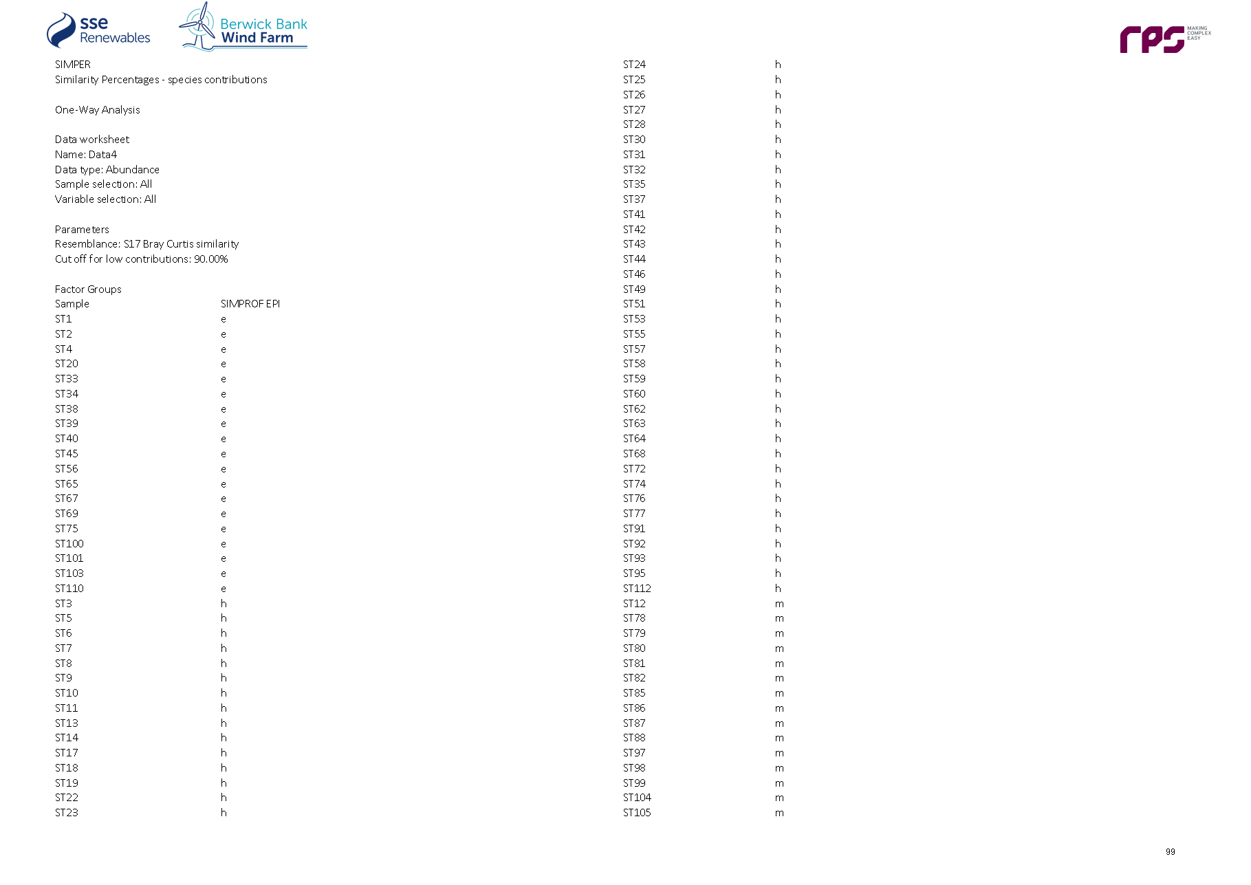
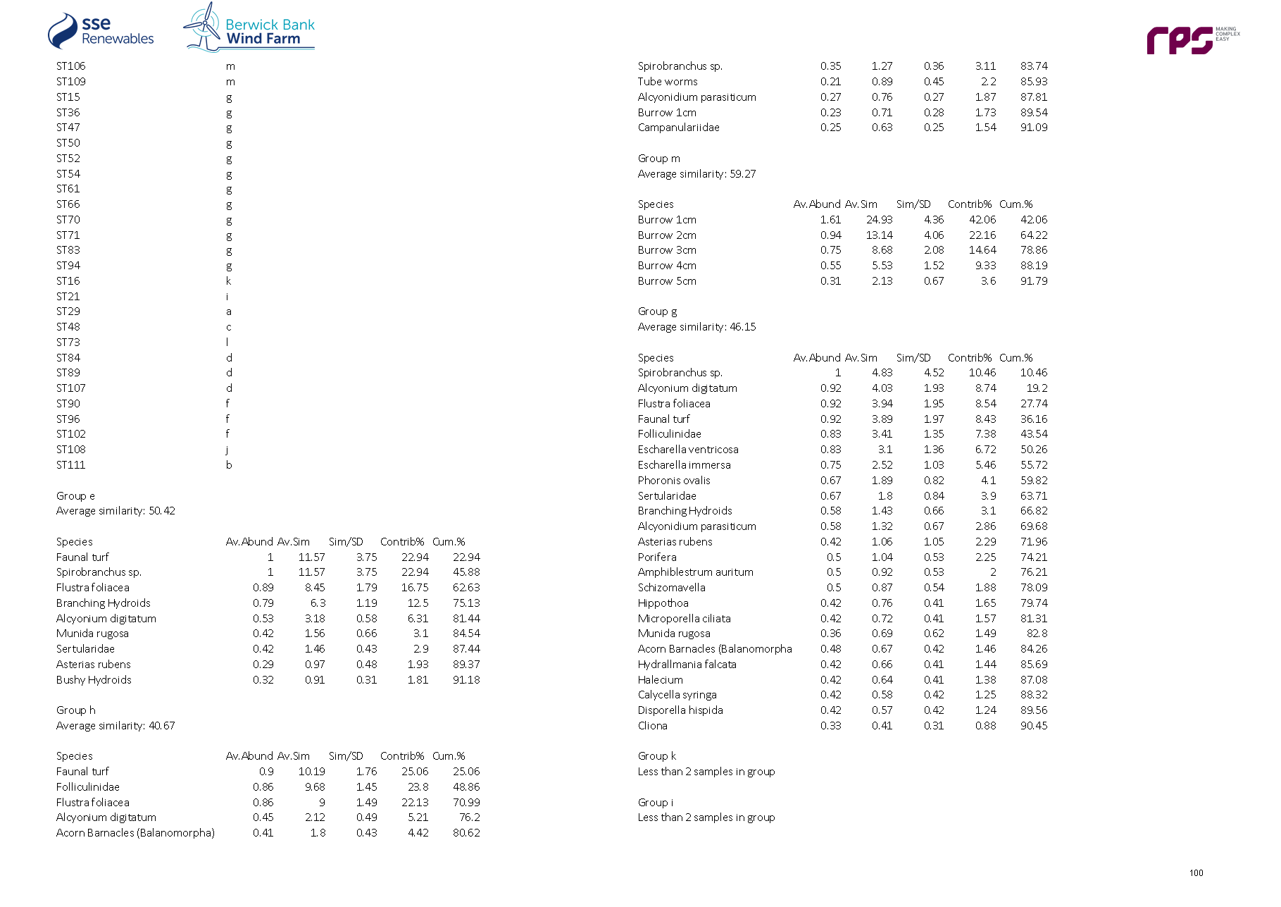
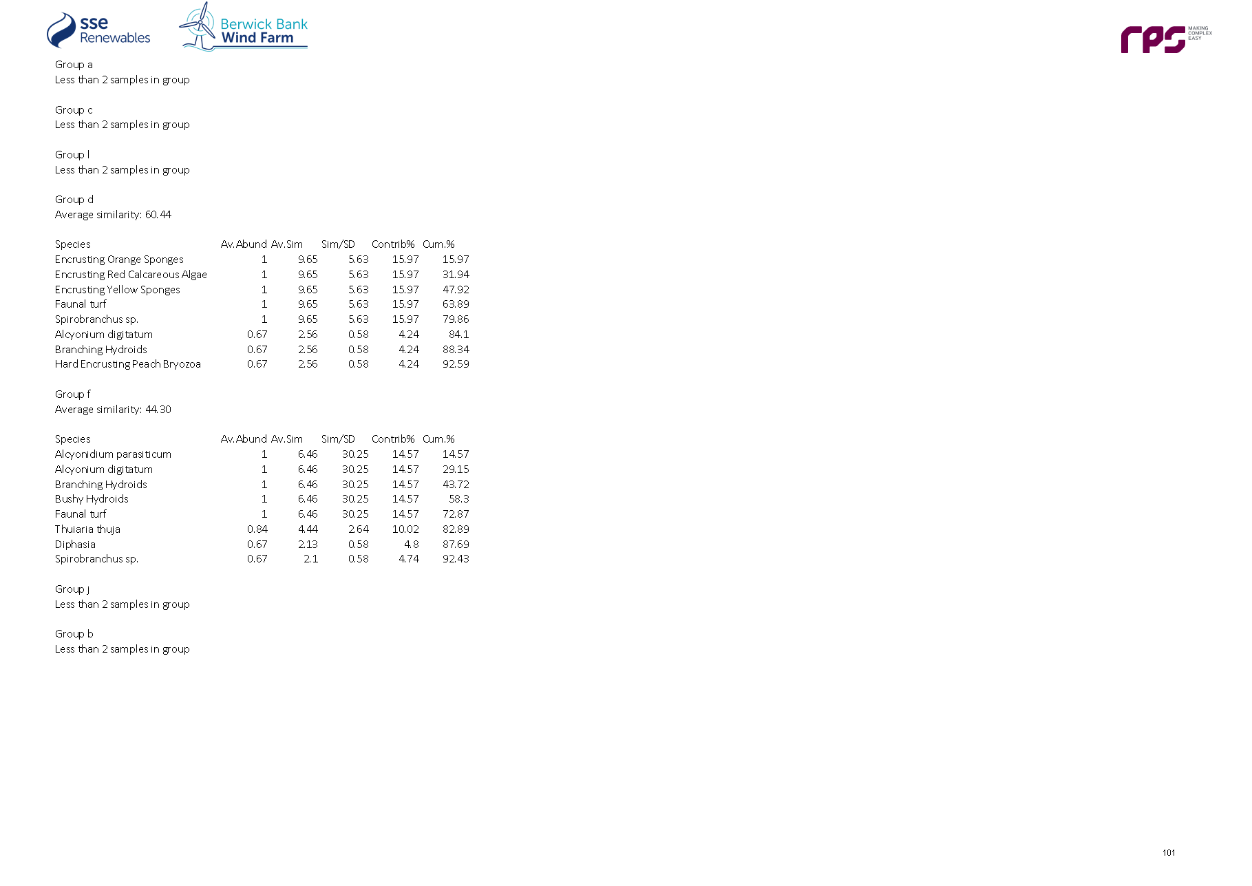
6.7. Annex G: Benthic Grab and DDV Epifaunal Data Univariate Analysis Results
6.7. Annex G: Benthic Grab and DDV Epifaunal Data Univariate Analysis Results
- S = number of species; N = abundance; B = Biomass (ash free dry mass in grams); d = Margalef’s index of Richness; J’ = Pielou’s Evenness index; H’ = Shannon-Wiener Diversity index; = Simpson’s Dominance index.
Sample Station | Preliminary Epifaunal Biotope | S | N | d | J’ | H’ | |
|---|---|---|---|---|---|---|---|
1 | SS.SCS.CCS | 11 | 6.416667 | 5.379529 | 0.842512 | 2.020256 | 0.853432 |
2 | SS.SCS.CCS | 21 | 12.42857 | 7.936514 | 0.911758 | 2.775868 | 0.929845 |
3 | SS.SCS.CCS | 10 | 9 | 4.096077 | 0.972424 | 2.239088 | 0.89159 |
4 | SS.SCS.CCS | 13 | 7.428571 | 5.984042 | 0.892613 | 2.289506 | 0.884615 |
5 | SS.SCS.CCS | 14 | 11.6 | 5.303947 | 0.955758 | 2.522301 | 0.916914 |
6 | SS.SCS.CCS | 6 | 5.166667 | 3.044645 | 0.948803 | 1.700026 | 0.811655 |
7 | SS.SCS.CCS | 15 | 10 | 6.080123 | 0.914818 | 2.477372 | 0.908163 |
8 | SS.SCS.CCS | 15 | 11.875 | 5.657856 | 0.948759 | 2.569287 | 0.919889 |
9 | SS.SCS.CCS | 8 | 6.222222 | 3.829055 | 0.916881 | 1.906599 | 0.844388 |
10 | SS.SCS.CCS | 13 | 9.8 | 5.257664 | 0.931104 | 2.388234 | 0.903374 |
11 | SS.SCS.CCS | 13 | 10.66667 | 5.069444 | 0.959523 | 2.461128 | 0.910807 |
12 | SS.SSa.CMuSa | 5 | 5.25 | 2.412213 | 0.5906 | 0.950534 | 0.481859 |
13 | SS.SCS.CCS | 5 | 3.5 | 3.192942 | 0.896409 | 1.442715 | 0.743764 |
14 | SS.SCS.CCS | 4 | 4.333333 | 2.045914 | 0.993887 | 1.37782 | 0.745562 |
15 | SS.SCS.CCS | 22 | 18.57143 | 7.187782 | 0.9547 | 2.951018 | 0.944615 |
16 | SS.SCS.CCS | 5 | 3.666667 | 3.078621 | 0.929445 | 1.495884 | 0.764463 |
17 | SS.SCS.CCS | 8 | 7.142857 | 3.560325 | 0.964216 | 2.005031 | 0.8624 |
18 | SS.SCS.CCS | 10 | 8 | 4.328085 | 0.960358 | 2.211307 | 0.885 |
19 | SS.SCS.CCS | 6 | 4.333333 | 3.409857 | 0.895301 | 1.604165 | 0.784024 |
20 | SS.SCS.CCS | 18 | 13.71429 | 6.49242 | 0.914834 | 2.64421 | 0.921007 |
21 | SS.SCS.CCS | 5 | 2.666667 | 4.078182 | 0.83391 | 1.342126 | 0.695313 |
22 | SS.SCS.CCS | 9 | 7.285714 | 4.028369 | 0.938559 | 2.062226 | 0.867359 |
23 | SS.SCS.CCS | 10 | 9.2 | 4.055509 | 0.978983 | 2.254191 | 0.893195 |
24 | SS.SCS.CCS | 6 | 5.25 | 3.015267 | 0.962318 | 1.724242 | 0.816327 |
25 | SS.SCS.CCS | 5 | 4.25 | 2.764495 | 0.949689 | 1.528466 | 0.775087 |
26 | SS.SCS.CCS | 9 | 9 | 3.640957 | 1 | 2.197225 | 0.888889 |
27 | SS.SCS.CCS | 8 | 7.125 | 3.564863 | 0.961841 | 2.000091 | 0.861804 |
28 | SS.SCS.CCS | 9 | 9 | 3.640957 | 1 | 2.197225 | 0.888889 |
29 | SS.SSa.OSa | 1 | 1 | - | - | 0 | 0 |
30 | SS.SCS.CCS | 9 | 8.142857 | 3.814717 | 0.969987 | 2.13128 | 0.87904 |
31 | SS.SCS.CCS | 11 | 9.428571 | 4.456835 | 0.963841 | 2.311191 | 0.897612 |
32 | SS.SCS.CCS | 14 | 12.28571 | 5.18251 | 0.967653 | 2.553691 | 0.920227 |
33 | SS.SCS.CCS | 19 | 9.669641 | 7.933041 | 0.829467 | 2.442314 | 0.903151 |
34 | SS.SCS.CCS | 5 | 4.333333 | 2.727886 | 0.963595 | 1.550846 | 0.781065 |
35 | SS.SCS.CCS | 7 | 5.4 | 3.557877 | 0.927903 | 1.805617 | 0.825789 |
36 | SS.SCS.CCS | 31 | 29.6 | 8.855371 | 0.964982 | 3.313736 | 0.959939 |
37 | SS.SCS.CCS | 10 | 8.333333 | 4.244755 | 0.963385 | 2.218275 | 0.8872 |
38 | SS.SCS.CCS | 14 | 9.714286 | 5.717811 | 0.924008 | 2.43851 | 0.905709 |
39 | SS.SCS.CCS | 6 | 5.166667 | 3.044645 | 0.948803 | 1.700026 | 0.811655 |
40 | SS.SCS.CCS | 9 | 7.333333 | 4.015197 | 0.943861 | 2.073874 | 0.868802 |
41 | SS.SCS.CCS | 10 | 7.285714 | 4.531915 | 0.931276 | 2.144341 | 0.875048 |
42 | SS.SCS.CCS | 6 | 5.666667 | 2.882507 | 0.994722 | 1.782303 | 0.83045 |
43 | SS.SCS.CCS | 4 | 4 | 2.164043 | 1 | 1.386294 | 0.75 |
44 | SS.SCS.CCS | 17 | 14 | 6.062771 | 0.962053 | 2.725701 | 0.93192 |
45 | SS.SCS.CCS | 11 | 8.666667 | 4.630735 | 0.946936 | 2.270652 | 0.891272 |
46 | SS.SCS.CCS | 7 | 7 | 3.08339 | 1 | 1.94591 | 0.857143 |
47 | SS.SCS.CCS | 20 | 14 | 7.19954 | 0.927336 | 2.778051 | 0.932945 |
48 | SS.SCS.CCS | 3 | 3 | 1.820478 | 1 | 1.098612 | 0.666667 |
49 | SS.SCS.CCS | 16 | 14.28571 | 5.640667 | 0.973162 | 2.698178 | 0.9312 |
50 | SS.SCS.CCS | 28 | 24.71429 | 8.418082 | 0.977013 | 3.255608 | 0.960473 |
51 | SS.SCS.CCS | 13 | 8.75 | 5.532366 | 0.876313 | 2.247698 | 0.878776 |
52 | SS.SCS.CCS | 24 | 24.875 | 7.156496 | 0.938379 | 2.982217 | 0.933966 |
53 | SS.SCS.CCS | 6 | 3.2 | 4.298669 | 0.889295 | 1.593403 | 0.765625 |
54 | SS.SCS.CCS | 29 | 26.5 | 8.544023 | 0.988446 | 3.328389 | 0.96349 |
55 | SS.SCS.CCS | 12 | 9 | 5.006316 | 0.961492 | 2.389217 | 0.902716 |
56 | SS.SCS.CCS | 17 | 11.42857 | 6.56783 | 0.931282 | 2.63852 | 0.9225 |
57 | SS.SCS.CCS | 16 | 14.33333 | 5.633617 | 0.975354 | 2.704257 | 0.931585 |
58 | SS.SCS.CCS | 5 | 4.333333 | 2.727886 | 0.963595 | 1.550846 | 0.781065 |
59 | SS.SCS.CCS | 2 | 2 | 1.442695 | 1 | 0.693147 | 0.5 |
60 | SS.SCS.CCS | 10 | 10 | 3.90865 | 1 | 2.302585 | 0.9 |
61 | SS.SCS.CCS | 17 | 13.16667 | 6.207112 | 0.95346 | 2.701356 | 0.929018 |
62 | SS.SCS.CCS | 14 | 13.16667 | 5.043278 | 0.98534 | 2.600369 | 0.924852 |
63 | SS.SCS.CCS | 10 | 9.285714 | 4.038632 | 0.984556 | 2.267024 | 0.894675 |
64 | SS.SCS.CCS | 7 | 4.285714 | 4.122897 | 0.905387 | 1.761801 | 0.808889 |
65 | SS.SCS.CCS | 8 | 5.833333 | 3.96918 | 0.890341 | 1.851412 | 0.827755 |
66 | SS.SCS.CCS | 24 | 20.14286 | 7.659391 | 0.967236 | 3.073928 | 0.952165 |
67 | SS.SCS.CCS | 11 | 5.875 | 5.647465 | 0.855298 | 2.050914 | 0.851064 |
68 | SS.SCS.CCS | 11 | 9 | 4.551196 | 0.963179 | 2.309603 | 0.896433 |
69 | SS.SCS.CCS | 20 | 12.75299 | 7.463373 | 0.83262 | 2.494306 | 0.89336 |
70 | SS.SCS.CCS | 29 | 27.42857 | 8.455165 | 0.990341 | 3.33477 | 0.963976 |
71 | SS.SCS.CCS | 29 | 28.16667 | 8.387907 | 0.99449 | 3.348741 | 0.964672 |
72 | SS.SCS.CCS | 6 | 5.111111 | 3.064821 | 0.93717 | 1.679183 | 0.808129 |
73 | SS.SCS.CCS | 10 | 6.111111 | 4.972077 | 0.888929 | 2.046834 | 0.856198 |
74 | SS.SCS.CCS | 11 | 5.285714 | 6.005978 | 0.854608 | 2.049261 | 0.845873 |
75 | SS.SCS.CCS | 14 | 7 | 6.680678 | 0.89442 | 2.360426 | 0.887963 |
76 | SS.SCS.CCS | 12 | 11.16667 | 4.558767 | 0.981798 | 2.439676 | 0.911562 |
77 | SS.SCS.CCS | 10 | 6.444444 | 4.830352 | 0.874995 | 2.014751 | 0.85434 |
78 | SS.SMu.CFiMu.SpnMeg | 5 | 5.888889 | 2.255977 | 0.841471 | 1.354295 | 0.706301 |
79 | SS.SMu.CFiMu.SpnMeg | 9 | 4.5 | 5.318875 | 0.821707 | 1.805474 | 0.773663 |
80 | SS.SMu.CFiMu.SpnMeg | 12 | 8 | 5.289882 | 0.874064 | 2.171967 | 0.858125 |
81 | SS.SMu.CFiMu.SpnMeg | 10 | 8.214286 | 4.273758 | 0.802211 | 1.84716 | 0.795766 |
82 | SS.SMu.CFiMu.SpnMeg | 11 | 5 | 6.213349 | 0.751689 | 1.802471 | 0.772893 |
83 | SS.SCS.CCS | 19 | 15.85714 | 6.513196 | 0.956794 | 2.817221 | 0.936775 |
84 | CR.MCR.EcCr | 6 | 5.666667 | 2.882507 | 0.994722 | 1.782303 | 0.83045 |
85 | SS.SMu.CFiMu.SpnMeg | 6 | 4 | 3.606738 | 0.685 | 1.227355 | 0.584877 |
86 | SS.SMu.CFiMu.SpnMeg | 8 | 8.6 | 3.253148 | 0.75765 | 1.575488 | 0.731206 |
87 | SS.SMu.CFiMu.SpnMeg | 13 | 8.125 | 5.728072 | 0.87558 | 2.245819 | 0.870533 |
88 | SS.SMu.CFiMu.SpnMeg | 9 | 7.75 | 3.906836 | 0.687007 | 1.509509 | 0.677419 |
89 | CR.MCR.EcCr | 16 | 11.54286 | 6.132294 | 0.924423 | 2.563045 | 0.919567 |
90 | SS.SCS.CCS | 18 | 16.125 | 6.114292 | 0.975603 | 2.819856 | 0.939246 |
91 | SS.SCS.CCS | 6 | 6 | 2.790553 | 0.859192 | 1.539465 | 0.747166 |
92 | SS.SCS.CCS | 9 | 8.125 | 3.818715 | 0.968011 | 2.126937 | 0.87858 |
93 | SS.SCS.CCS | 5 | 3.5 | 3.192942 | 0.901436 | 1.450805 | 0.744898 |
94 | SS.SCS.CCS | 11 | 9.375 | 4.468182 | 0.960317 | 2.30274 | 0.896711 |
95 | SS.SCS.CCS | 9 | 7.571429 | 3.951824 | 0.964367 | 2.11893 | 0.875044 |
96 | SS.SCS.CCS | 18 | 13.44444 | 6.54207 | 0.940552 | 2.718546 | 0.930264 |
97 | SS.SMu.CFiMu.SpnMeg | 5 | 4.6 | 2.621135 | 0.66359 | 1.068006 | 0.533081 |
98 | SS.SMu.CFiMu.SpnMeg | 7 | 7 | 3.08339 | 0.705072 | 1.372007 | 0.69035 |
99 | SS.SMu.CFiMu.SpnMeg | 10 | 7.153846 | 4.573984 | 0.845113 | 1.945945 | 0.820904 |
100 | SS.SCS.CCS | 13 | 7 | 6.16678 | 0.85184 | 2.184927 | 0.872553 |
101 | SS.SCS.CCS | 18 | 7.866667 | 8.241887 | 0.808713 | 2.337482 | 0.885665 |
102 | SS.SCS.CCS | 23 | 13.14391 | 8.540511 | 0.874795 | 2.742914 | 0.929418 |
103 | SS.SCS.CCS | 8 | 7 | 3.597288 | 0.958118 | 1.992351 | 0.860816 |
104 | SS.SMu.CFiMu.SpnMeg | 5 | 4 | 2.88539 | 0.762854 | 1.227767 | 0.632653 |
105 | SS.SMu.CFiMu.SpnMeg | 6 | 4.222222 | 3.471351 | 0.739821 | 1.325581 | 0.66482 |
106 | SS.SMu.CFiMu.SpnMeg | 7 | 7.5 | 2.977811 | 0.553213 | 1.076502 | 0.538311 |
107 | CR.MCR.EcCr | 18 | 12.0303 | 6.834367 | 0.903115 | 2.610337 | 0.920937 |
108 | SS.SSa.IFiSa | 1 | 1.266667 | 0 |
| 0 | 0 |
109 | SS.SMu.CFiMu.SpnMeg | 10 | 4.818182 | 5.723747 | 0.726866 | 1.673671 | 0.722677 |
110 | SS.SCS.CCS | 6 | 2.941176 | 4.634738 | 0.759775 | 1.361334 | 0.7088 |
111 | CR.MCR.EcCr | 17 | 13.85 | 6.087619 | 0.952986 | 2.700013 | 0.93047 |
112 | SS.SCS.CCS | 6 | 5.333333 | 2.9869 | 0.972586 | 1.74264 | 0.820313 |
6.8. Annex H: Benthic Trawls Epifaunal Data Multivariate Analysis Results
6.8. Annex H: Benthic Trawls Epifaunal Data Multivariate Analysis Results
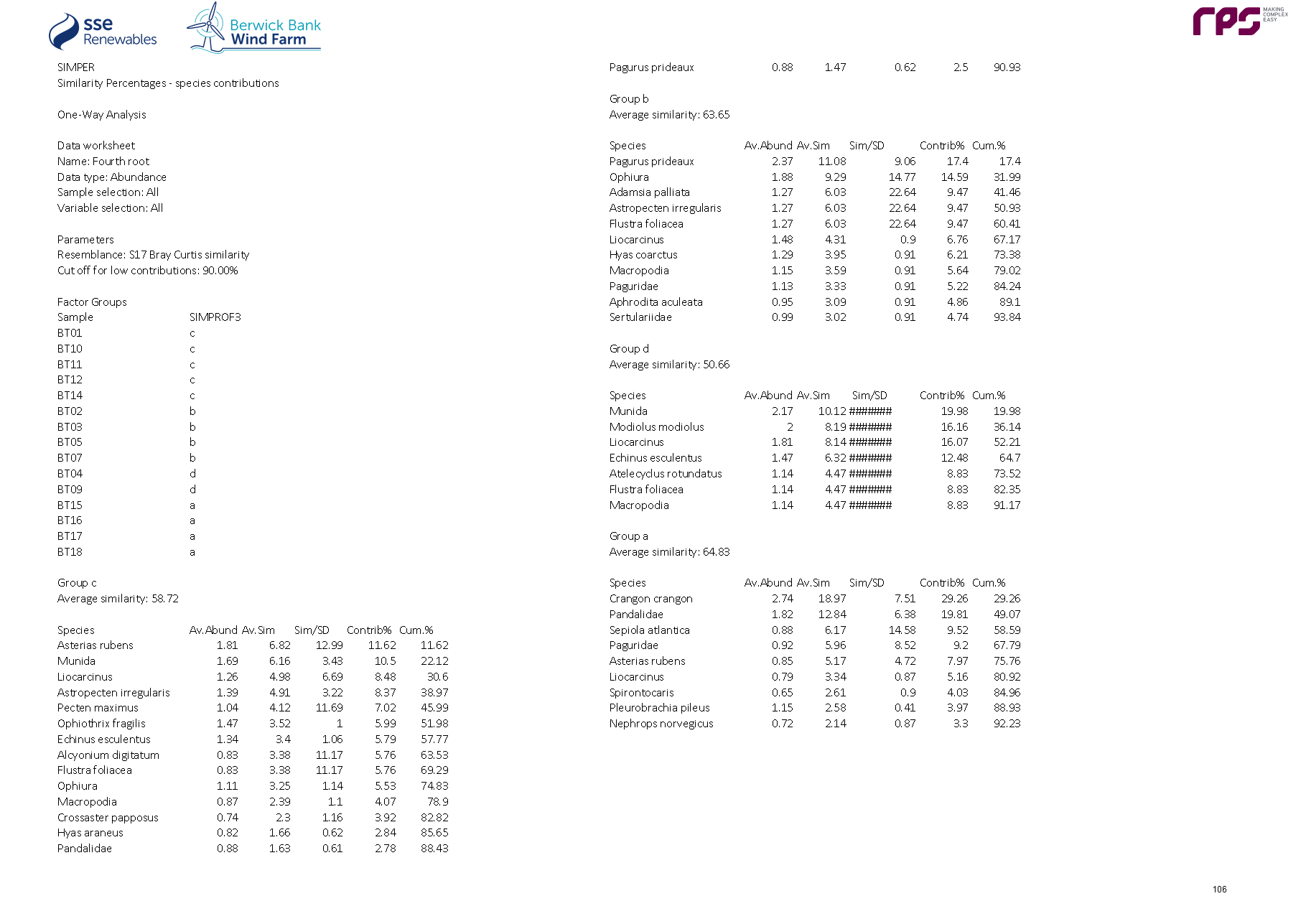
6.9. Annex I: Benthic Trawls Epifaunal Data Univariate Analysis Results
6.9. Annex I: Benthic Trawls Epifaunal Data Univariate Analysis Results
- S = number of species; N = abundance; B = Biomass (ash free dry mass in grams); d = Margalef’s index of Richness; J’ = Pielou’s Evenness index; H’ = Shannon-Wiener Diversity index; = Simpson’s Dominance index.
Sample Station | Preliminary Epifaunal Biotope | S | N | d | J’ | H’ | |
|---|---|---|---|---|---|---|---|
1 | SS.SCS.CCS | 15 | 103 | 3.020673 | 0.779095 | 2.109828 | 0.837214 |
2 | SS.SCS.CCS | 11 | 21 | 3.284587 | 0.935662 | 2.243619 | 0.879819 |
3 | SS.SCS.CCS | 12 | 62 | 2.665288 | 0.611081 | 1.51848 | 0.627992 |
4 | SS.SCS.CCS | 13 | 32 | 3.462468 | 0.925512 | 2.373891 | 0.888672 |
5 | SS.SCS.CCS | 15 | 41 | 3.769955 | 0.839882 | 2.274442 | 0.848305 |
7 | SS.SCS.CCS | 14 | 46 | 3.39546 | 0.734093 | 1.937314 | 0.782609 |
9 | SS.SCS.CCS | 17 | 120 | 3.342042 | 0.697672 | 1.976654 | 0.813472 |
10 | SS.SCS.CCS | 18 | 384 | 2.856834 | 0.610374 | 1.764207 | 0.699409 |
14 | SS.SCS.CCS | 19 | 169 | 3.508841 | 0.763826 | 2.249038 | 0.855992 |
11 | SS.SMx.CMx.FluHyd | 21 | 326 | 3.456083 | 0.530509 | 1.615145 | 0.60659 |
12 | SS.SMx.CMx.FluHyd | 19 | 198 | 3.403762 | 0.497326 | 1.464345 | 0.561983 |
15 | SS.SSa.CMuSa | 11 | 1076 | 1.432458 | 0.329307 | 0.789644 | 0.380936 |
16 | SS.SSa.CMuSa | 7 | 307 | 1.047697 | 0.51851 | 1.008974 | 0.522637 |
17 | SS.SSa.CMuSa | 13 | 1183 | 1.695919 | 0.271659 | 0.696792 | 0.289103 |
18 | SS.SSa.CMuSa | 15 | 1294 | 1.953808 | 0.407393 | 1.103241 | 0.496321 |
6.10. Annex J: Sediment Contamination Results
6.10. Annex J: Sediment Contamination Results
6.10.1. Concentrations of PCBs Recorded in Sediments within the Proposed Development Benthic Subtidal and Intertidal Ecology Study Area
Description (PCBs) | 28 | 52 | 101 | 118 | 138 | 153 | 180 | Sum of ICES 7 |
Units | mg/kg | mg/kg | mg/kg | mg/kg | mg/kg | mg/kg | mg/kg | mg/kg |
MS AL1 (mg/kg) | - | - | - | - | - | - | - | 0.02 |
MS AL2 (mg/kg) | - | - | - | - | - | - | - | 0.18 |
Sample No. |
|
|
|
|
|
|
|
|
ST91 | <0.0001 | <0.0002 | <0.0002 | <0.0002 | <0.0002 | <0.0002 | <0.0002 | <0.0013 |
ST92 | <0.0001 | <0.0002 | <0.0002 | <0.0002 | <0.0002 | <0.0002 | <0.0002 | <0.0013 |
ST93 | <0.0001 | <0.0002 | <0.0002 | <0.0002 | <0.0002 | <0.0002 | <0.0002 | <0.0013 |
ST94 | <0.0001 | <0.0002 | <0.0002 | <0.0002 | <0.0002 | <0.0002 | <0.0002 | <0.0013 |
ST95 | <0.0001 | <0.0002 | <0.0002 | <0.0002 | <0.0002 | <0.0002 | <0.0002 | <0.0013 |
ST96 | <0.0001 | <0.0002 | <0.0002 | <0.0002 | <0.0002 | <0.0002 | <0.0002 | <0.0013 |
ST97 | <0.0001 | <0.0002 | <0.0002 | <0.0002 | <0.0002 | <0.0002 | <0.0002 | <0.0013 |
ST98 | <0.0001 | <0.0002 | <0.0002 | <0.0002 | <0.0002 | <0.0002 | <0.0002 | <0.0013 |
ST99 | <0.0001 | <0.0002 | <0.0002 | <0.0002 | <0.0002 | <0.0002 | <0.0002 | <0.0013 |
6.10.2. Concentrations of PAHs Recorded in Sediment within the Proposed Development Benthic Subtidal and Intertidal Ecology Study Area
Description (PAH) | Naphthalene | Acenaphthylene | Acenaphthene | Fluorene | Phenanthrene | Anthracene |
Units | mg/kg | mg/kg | mg/kg | mg/kg | mg/kg | mg/kg |
MS AL1 (mg/kg) | 0.1 | 0.1 | 0.1 | 0.1 | 0.1 | 0.1 |
MS AL2 (mg/kg) | n/a | n/a | n/a | n/a | n/a | n/a |
Canadian TEL (mg/kg) | 0.0346 | 0.00587 | 0.00671 | 0.0212 | 0.0867 | 0.0469 |
Canadian PEL (mg/kg) | 0.391 | 0.128 | 0.0889 | 0.144 | 0.544 | 0.245 |
Sample No. |
|
|
|
|
|
|
Sample 91 | <0.0026 | <0.002 | <0.0017 | <0.0016 | <0.00390 | <0.0024 |
Sample 92 | <0.0026 | <0.002 | <0.0017 | <0.0016 | <0.00390 | <0.0024 |
Sample 93 | <0.0026 | <0.002 | <0.0017 | <0.0016 | <0.00390 | <0.0024 |
Sample 94 | <0.0026 | <0.002 | <0.0017 | <0.0016 | <0.00390 | <0.0024 |
Sample 95 | <0.0026 | <0.002 | <0.0017 | <0.0016 | <0.00390 | <0.0024 |
Sample 96 | <0.0026 | <0.002 | <0.0017 | <0.0016 | <0.00390 | <0.0024 |
Sample 97 | <0.0026 | <0.002 | <0.0017 | <0.0016 | <0.00390 | <0.0024 |
Sample 98 | 0.00445 | <0.002 | <0.0017 | <0.0016 | 0.01010 | <0.0024 |
Sample 99 | 0.00764 | <0.002 | <0.0017 | 0.00293 | 0.01890 | 0.00377 |
Description (PAH) | Fluoranthene | Pyrene | Benzo(a)anthracene | Chrysene | Benzo(b)fluoranthene | Benzo(k)fluoranthene |
Units | mg/kg | mg/kg | mg/kg | mg/kg | mg/kg | mg/kg |
MS AL1 (mg/kg) | 0.1 | 0.1 | 0.1 | 0.1 | 0.1 | 0.1 |
MS AL2 (mg/kg) | n/a | n/a | n/a | n/a | n/a | n/a |
Canadian TEL (mg/kg) | 0.113 | 0.153 | 0.074 | 0.108 | n/a | n/a |
Canadian PEL (mg/kg) | 1.494 | 1.398 | 0.693 | 0.846 | n/a | n/a |
Sample No. |
|
|
|
|
|
|
Sample 91 | <0.0024 | <0.00280 | <0.0016 | <0.0017 | 0.00402 | <0.002 |
Sample 92 | <0.0024 | <0.00280 | <0.0016 | <0.0017 | 0.00223 | <0.002 |
Sample 93 | <0.0024 | <0.00280 | <0.0016 | <0.0017 | 0.00286 | <0.002 |
Sample 94 | <0.0024 | <0.00280 | <0.0016 | <0.0017 | <0.0016 | <0.002 |
Sample 95 | <0.0024 | <0.00280 | <0.0016 | <0.0017 | 0.00468 | <0.002 |
Sample 96 | <0.0024 | <0.00280 | <0.0016 | <0.0017 | 0.00316 | <0.002 |
Sample 97 | 0.00429 | <0.00280 | 0.00241 | <0.0017 | 0.00987 | 0.00267 |
Sample 98 | 0.01210 | 0.01100 | 0.00725 | 0.00549 | 0.02430 | 0.00766 |
Sample 99 | 0.02100 | 0.01930 | 0.01300 | 0.01050 | 0.04210 | 0.01150 |
Description (PAH) | Benzo(a)pyrene | Indeno(1,2,3-c,d)pyrene | Dibenzo(a,h)anthracene | Benzo(g,h,i)perylene |
|
|
Units | mg/kg | mg/kg | mg/kg | mg/kg |
|
|
MS AL1 (mg/kg) | 0.1 | 0.1 | 0.01 | 0.1 |
|
|
MS AL2 (mg/kg) | n/a | n/a | n/a | n/a |
|
|
Canadian TEL (mg/kg) | 0.0888 | n/a | 0.00622 | n/a |
|
|
Canadian PEL (mg/kg) | 0.763 | n/a | 0.135 | n/a |
|
|
Sample No. |
|
|
|
|
|
|
Sample 91 | 0.00118 | 0.00388 | <0.0016 | 0.00398 |
|
|
Sample 92 | <0.0009 | <0.0022 | <0.0016 | 0.00191 |
|
|
Sample 93 | <0.0009 | <0.0022 | <0.0016 | 0.00254 |
|
|
Sample 94 | <0.0009 | <0.0022 | <0.0016 | <0.0014 |
|
|
Sample 95 | 0.00140 | 0.00394 | <0.0016 | 0.00397 |
|
|
Sample 96 | <0.0009 | 0.00298 | <0.0016 | 0.00292 |
|
|
Sample 97 | 0.00329 | 0.00785 | <0.0016 | 0.00810 |
|
|
Sample 98 | 0.00883 | 0.01820 | 0.00381 | 0.01890 |
|
|
Sample 99 | 0.0166 | 0.02870 | 0.00610 | 0.03000 |
|
|
6.11. Annex K: Intertidal Biotopes
6.11. Annex K: Intertidal Biotopes
6.11.1. Littoral Biotopes at the Skateraw Landfall
Shore Position | Biotope | Biotope Name | Biotope Description from the Skateraw Landfall |
|---|---|---|---|
Upper shore | LR | Littoral rock (and other hard substrata) | Barren bedrock with no species recorded mainly occurring at MHWS and areas of elevated bedrock. |
Upper shore | LR.FLR.Lic.YG | Yellow and grey lichens on supralittoral rock | Biotope present at the Skateraw Landfall as a scattered fringe and dominated by the yellow lichen X. parietina. |
Upper shore | LR.FLR.Lic.Ver | Verrucaria maura on littoral rock fringe | Biotope recorded as a scattered fringe on upper shore bedrock, boulders and cobbles and dominated by V. maura although a significant amount of rock was uncolonised. Enteromorpha intestinalis and L. saxatilis also present. |
Upper shore | LS.LSa.St.Tal | Talitrids on the upper shore and strand-line. | Biotope recorded at Stateraw Beach with talitrid amphipods occurring super abundantly under the decomposing seaweeds of the drift line. |
Upper shore | LR.FLR.Eph.Ent | Enteromorpha spp. on freshwater influenced and or unstable upper eulittoral rock | Biotope recorded on unstable rock in the upper shore and in areas influences by fresh water from the Dry Burn and was dominated by E. intestinalis. Other species presented included sparse patches of U. lactuca and occasional individuals of L. saxatilis. |
Upper shore | LR.FLR.Rkp.G | Green seaweeds (Enteromorpha spp. and Cladophora spp.) in shallow upper shore rockpools | Biotope recorded in rockpools within the LR.FLR.Eph.Ent biotope and had a similar species assemblage. |
Upper shore | LR.LLR.FVS.PelVS | Pelvetia canaliculata on sheltered variable salinity littoral fringe rock | Biotope recorded in occasional patches within the LR.LLR.F.Fspi.X biotope where P. canaliculata was dominant on its landward fringe. This biotope contained the same associate species as Fspi.X (see below). |
Upper shore | LR.LLR.F.Fspi.X | Fucus spiralis on full salinity upper eulittoral mixed substrata | Biotope dominated by F. spiralis with abundant V. maura. Other species occurring occasionally were E. intestinalis, S. balanoides, P. vulgata, L. saxatilis and L. littorea. Species assemblage was the same as that associated with the LR.LLR.F.Fspi.B biotope. |
Upper shore | LR.LLR.F.Fspi.B | Fucus spiralis on exposed to moderately exposed upper eulittoral rock | Biotope dominated by F. spiralis with abundant V. maura. Other species occurring occasionally were E. intestinalis, S. balanoides, P. vulgata, L. saxatilis and L. littorea. Species assemblage was the same as that associated with the LR.LLR.F.Fspi.X biotope. |
Mid shore | LR.LLR.F.Fves | Fucus vesiculosus on moderately exposed to sheltered mid eulittoral rock | Biotope characterised by a continuous canopy of F. vesiculosus and sparse occurences of S. balanoides. Species including C. pagurus and C. maenas were occasionally present under rocks. This community was differentiated into two variants which largely had the same species assemblages: LR.LLR.F.Fves.X and LR.LLR.F.Fves.FS (see below). |
Mid shore | LR.LLR.F.Fves.FS | Fucus vesiculosus on full salinity moderately exposed to sheltered mid eulittoral rock | Biotope occurred on boulders and bedrock with a species assemblage as described above for LR.LLR.F.Fves. |
Mid shore | LR.HLR.MusB.Sem.Sem | Semibalanus balanoides, Patella vulgata and Littorina spp. on exposed to moderately exposed or sheltered vertical eulittoral rock | Biotope occurred on bedrock and boulders and was dominated by S. balanoides which was present in super abundant numbers. Species recorded occasionally included P. vulgata, L. littorea, L. obtusata, N. lapillus and V. maura. Distributions of algae such as F. vesiculosus, P. purpurea and E. intestinalis were sparse within this biotope. |
Mid shore | LR.MLR.BF.FvesB | Fucus vesiculosus and barnacle mosaics on moderately exposed mid eulittoral rock | Biotope recorded predominantly on mixed rocky sediments dominated by boulders and also on bedrock. Species assemblage dominated by F. vesiculosus and S. balanoides. Ascophyllum nodosum was occasionally present with V. lanosa attached. The red seaweeds M. stellatus and C. officinalis were occasionally present along with fauna including P. vulgata, L. littorea, L. obtusata, C. maenas and A. equina. Juvenile M. edulis were rarely observed. |
Mid shore | LR.HLR.FR.Coff.Coff | Corallina officinalis and Mastocarpus stellatus on exposed to moderately exposed lower eulittoral rock | Biotope dominated by C. officinalis and coralline crusts with abundant V. fucoides. Other algae commonly recorded included C. rupestris and F. vesiculosus whilst L. difformis and M. stellatus were only occasionally recorded. Variable densities of L. littorea were also recorded. This biotope contained numerous shallow coralline rock pools with flat rocks under which a diverse assemblage of species occurred. |
Mid shore | LR.LLR.F.Fves.X | Fucus vesiculosus on mid eulittoral mixed substrata | Biotope occurred on substrate with a higher proportion of cobbles and pebbles with a species assemblage as described above for LR.LLR.F.Fves. |
Mid shore | LR.FLR.Rkp.Cor.Cor | Corallina officinalis and coralline crusts in shallow eulittoral Rockpools | Biotope occurred from the middle of the shore up to the F. spiralis zone within the numerous rockpools present at this landfall. Coralline crusts and C. officinalis were dominant with C. rupestris and H. siliquosa frequently recorded. Other seaweeds including M. stellatus, C. crispus, Ceramium sp. and U. lactuca occurred occasionally with a scattering of F. vesiculosus and P. vulgata. A diverse range of invertebrate animals occurred including L. littorea, C. pagurus, G. cineraria, S. spirorbis, P. bernhardus and C. maenas. Also present in very low abundances were U. felina, S. unicornis, L. nivea, D. grossularia and D. pseudoargus. |
Lower shore | LR.MLR.BF.Fser | Fucus serratus on moderately exposed lower eulittoral rock | Biotope commonly recorded on the lower shore containing a canopy of F. serratus predominantly on bedrock with frequent green seaweeds underneath such as C. rupestris. Invertebrates recorded included S. balanoides, P. vulgata and N. lapillus, particularly in rock crevices. Two variants of this biotope (Fser.R and Fser.Bo) were fairly widespread (see below). |
Lower shore | LR.MLR.BF.Fser.R | Fucus serratus and red seaweeds on moderately exposed lower eulittoral rock. | Biotope characterised by common occurrences of the red seaweeds M. stellatus, O. pinnatifida, C. officinalis and Ceramium sp. and occasional green seaweeds such as C. rupestris and E. intestinalis. Invertebrates including P. vulgata and S. balanoides were frequently recorded with occasional specimens of L. littorea, N. lapillus and C. maenas. |
Lower shore | LR.MLR.BF.Fser.Bo | Fucus serratus and under-boulder fauna on exposed to moderately exposed lower eulittoral boulders | Species rich biotope with super abundant F. serratus and occasionally F. vesiculosus. Red seaweeds included P. palmata, M. stellatus, O. pinnatifida, L. articulata, O. dentata, C. officinalis and calcareous encrusters. The faunal assemblage was also species rich with abundant N. puber, P. platycheles, C. maenas, C. pagurus and G. squamifera under most rocks. Other faunal species occasionally recorded included H. sanguinolenta, A. rubens, O. fragilis, P. miliaris and A. equina. Polychaetes were occasionally observed (e.g. E. viridis and P. triqueter) and gastropod molluscs (e.g. P. vulgata, N. lapillus, L. littoralis and G. cineraria) were present above and under boulders. The sea slug D. pseudoargus occurred infrequently under stones. The sponge H. panicea occurred abundantly while epiphytic colonies of the ascidian B. schlosseri and the bryozoans E. pilosa and M. membranacea were present both on fronds of F. serratus and on rocks. |
Lower shore | LR.MIR.KR.Ldig | Laminaria digitata on moderately exposed sublittoral fringe rock | Biotope recorded as a narrow fringe on vertical surfaces where rock platforms dropped off either into lower shore intertidal L. digitata boulder fields or directly into the sea. Biotope characterised by a similar suite of species as recorded in association with the LR.MLR.BF.Fser.Bo biotope (see above). |
Lower shore | LR.MIR.KR.Ldig.Bo | Laminaria digitata and under-boulder fauna on sublittoral fringe boulders | Biotope characterised by a similar suite of species as recorded in association with the LR.MLR.BF.Fser.Bo biotope (see above) but present lower down the shore and with the kelp L. digitata as the dominant species. Additional species only recorded in this biotope included the seaweeds S. latissima, L. hyperborea, D. carnosa and the gastropod T. monacha. |
Lower shore | LR.FLR.Rkp.FK | Fucoids and kelp in deep eulittoral rockpools | Biotope recorded within the rockpools present throughout the lower and lower mid shore zones. Fucus serratus and L. digitata dominated the deeper waters of the pools while C. officinalis and coralline crusts dominated the shallow fringes. Also frequently recorded were H. siliquosa, M. stellatus, C. crispus, P. palmata, A. plicata and Ceramium sp. with scattered N. lapillus, P. vulgata and A. equina. Shrimps Palaemon sp. occurred occasionally. |
Lower shore | LR.FLR.Rkp.SwSed | Seaweeds in sediment-floored eulittoral rockpools | Biotope recorded in deep pools although depth and suspended sediments hampered visibility. |
Lower shore | LS.LSa.MuSa.MacAre | Limecola (Macoma) balthica and Arenicola marina in littoral muddy sand | Biotope recorded in areas of fine muddy sand with M. balthica and M. tenuis were rarely observed in dig over sampling. Oligochaete worms and H. diversicolor, S. armiger and L. conchilega were recorded in low densities. Patches of this biotope were also recorded in large rockpools containing a layer of sediment at the base. |
Lower shore | LS.LSa.MuSa.Lan | Lanice conchilega in littoral sand | Biotope occurred predominantly in clean sand, mainly along the mid and lower shores in areas of dense populations of L. conchilega. Polychaetes E. lumbricoides, N. hombergii, S. armiger and A. marina were often present. |
Lower shore | LS.LSa.FiSa.Po | Polychaetes in littoral fine sand | Biotope was characterised by a similar suite of species as recorded within the LS.LSa.MuSa.MacAre and LS.LSa.MuSa.Lan biotopes with occasional occurrences of the polychaetes N. hombergii, P. fulgens, H. diversicolor and S. armiger. Arenicola marina was rarely present. |
[1] SACFOR classification scale, S=Superabundant, A=Abundant, C=Common, F=Frequent, O=Occasional and R=Rare.
[2] Although the • SS.SSa.CFiSa.ApriBatPo biotope is not within the Proposed Development benthic subtidal and intertidal ecology study area it has been included as an IEF due to its close proximity,