1. Introduction

Berwick Bank Wind Farm Limited (BBWFL), a wholly owned subsidiary of SSE Renewables Limited (hereafter be referred to as ‘the Applicant’), is proposing the development of the Berwick Bank Wind Farm (hereafter referred to as the ‘Proposed Development’), an offshore wind farm off the east coast of Scotland. The Proposed Development array area is located in the outer Firth of Forth and Forth of Tay, approximately 37.8 km east of the Scottish Borders coastline (St Abb’s Head) and 47.6 km from the East Lothian coastline. The Proposed Development array area will be connected to a SP Energy Networks (SPEN) substation at Branxton via a Proposed Development export cable corridor.
An Environmental Impact Assessment was (EIA) was carried out to determine the potential effects of the Proposed Development on sensitive marine mammal receptors from a range of different impacts. A key impact assessed was the potential for elevations in subsea noise during piling activities to lead to injury and behavioural disturbance to individuals. Subsea noise modelling was conducted to predict the potential spatial scale of the effect. In particular, for behavioural disturbance, the assessment predicted that the elevations in subsea noise leading to disturbance could extend over a considerable area and potentially affect a large number of individuals of the key species identified within the marine mammal study area.
Population modelling was therefore carried out to determine the potential for a short to medium term effects (piling could occur over a total duration of 372 days intermittently within a 52 month piling period during the eight year offshore construction timeframe) to result in long term population level effects on any species. The interim Population Consequences of Disturbance (iPCoD) model [1] (developed by Sea Mammal Research Unit (SMRU) Consulting, collaborating with a team of researchers at the University of St Andrews), was adopted to simulate the potential changes in the population over time and is explained within this report.

1.2. iPCoD

The iPCoD model simulates the changes in a population over time, for both a disturbed and an undisturbed population. This provides a comparison of the type of changes that could occur resulting from natural environmental variation, demographic stochasticity (i.e. variability in population growth rates) and disturbance (Harwood et al., 2014; King et al., 2015).
The iPCoD model is based on expert elicitation, a widely accepted process in conservation science whereby the opinions of many experts are combined when there is an urgent need for decisions to be made but a lack of empirical data with which to inform them (Donovan et al., 2016). In the case of the iPCoD model, the marine mammal experts were asked for their opinion on how changes in hearing resulting from Permanent Threshold Shift (PTS) and behavioural disturbance (equivalent to a score of 5* or higher on the ‘behavioural severity scale’ described by Southall et al. (2007)) associated with offshore renewable energy developments affect calf and juvenile survival, and the probability of giving birth (Harwood et al., 2014). Experts were asked to estimate values for two parameters which determine the shape of the relationships between the number of days of disturbance experienced by an individual and its vital rates, thus providing parameter values for functions that form part of the iPCoD model (Harwood et al., 2014). Following the initial development of the iPCoD model a study was undertaken to update the transfer functions on the effects of PTS and disturbance on the probability of survival and giving birth to a viable young for harbour porpoise, harbour seal and grey seal (again via expert elicitation) (Booth and Heinis, 2018; Booth et al., 2019). The iPCoD model has been updated in light of additional work undertaken since it was originally launched.
A potential limitation of the iPCoD model is that no form of density dependence has been incorporated due to the uncertainties as to how this may occur. As discussed in Harwood et al. (2014), the concept of density-dependence is fundamental to understanding how animal populations respond to a reduction in their size. In population biology, density-dependant factors, such as resource availability or competition for space, can limit population growth. If the population declines, these factors no longer become limiting and therefore, for the remaining individuals in a population, there is likely to be an increase in survival rate and reproduction. This then allows the population to expand back to previous levels at which density-dependant factors become limiting again (i.e. population remains at carrying capacity). The limitations for assuming a simple linear ratio between the maximum net productivity level and carrying capacity have been highlighted by Taylor and Master (1993) as simple models demonstrate that density dependence is likely to involve several biological parameters which themselves have biological limits (e.g. fecundity and survival). For UK populations of harbour porpoise (and other marine mammal species) however, there is no published evidence for density dependence and therefore, density dependence assumptions are not currently included within the iPCoD protocol.

2. Methodology

2.1. Piling Parameters

2.1.1. Maximum Design Scenario

The maximum design scenario for piling at the Proposed Development assumes that 5.5 m diameter piled jacket foundations will be installed using a maximum hammer energy of 4,000 kJ. This represents the absolute maximum energy likely to be required at any point across foundation installation. Taken as an average, the maximum hammer energy is likely to be no greater than 3,000 kJ. For the purposes of population modelling, the assessment focussed only on the absolute maximum of 4,000 kJ as this represented the maximum adverse design (as agreed by consultees at Marine Mammal Road Map Meeting 3, 18 January 2022).
Piling will be required at up to 179 wind turbine foundations and ten offshore substation platform (OSP)/Offshore convertor station platform foundations. The maximum design scenario was based on concurrent piling at wind turbine foundations with the largest separation between piling locations. Although piling could occur concurrently at a wind turbine and OSP/Offshore convertor station platform foundation these locations would be closer together compared to two wind turbine foundations. Therefore, piling at OSPs/Offshore convertor station platforms was considered as a single piling event and modelled as a separate operation within iPCoD but not coincident with concurrent piling at the wind turbine foundations (since this would represent three concurrent piling events which is not proposed as part of the Proposed Development design). Using the maximum number of hours of piling per pile, the number of piles likely to be installed within 24 hours and the number of concurrent installation vessels, it was possible to estimate the maximum number of days (24 hours) within which piling could occur on the basis of two piling operations:

287 piling days (concurrent vessel) for the 179 wind turbines; and
85 piling days (single vessel) for the ten OSPs/Offshore convertor station platforms.
1. It is estimated that piling activity at the Proposed Development will take place in three campaigns and an indicative piling construction schedule is provided in Table 2.1 Open ▸ . Piling could potentially take place at any point within the foundation installation phases; however, for the purposes of developing the piling programme for iPCoD (a requirement of the model) an indicative programme has been developed based on a realistic installation approach. Therefore, within each campaign, a realistic scenario has been assumed where there are nine months of piling followed by 12 months where jackets are installed over the piles.

2.1.2. Noise Modelling (Conversion Factors)

Subsea noise modelling was undertaken to predict the potential spatial scale of the effect of subsea noise. Potential injury, in the form of a PTS was determined using published and peer reviewed thresholds developed by Southall et al. (2019) for the dual metrics un-weighted peak Sound Pressure Levels (SPLpk) and marine mammal hearing-weighted cumulative Sound Exposure Level (SELcum). For behaviour disturbance a dose-response approach was undertaken using the metric single strike Sound Exposure Level (SELss) with contours modelled in 5 dB increments based on Graham et al. (2017). A full description of subsea noise modelling is provided in volume 3, appendix 10.1 and summarised in section 10.11.1 of volume 2, chapter 10. Further to discussion via the marine mammal Road Map process, the subsea noise modelling investigated the sensitivity of using different conversion factors to determine the amount of energy converted into received sound. In this respect, three conversion factors were modelled: 10% reducing to 1% as piling progresses, 4% reducing to 0.5% as piling progresses and a constant conversion factor of 1% throughout piling.
A detailed study of existing literature was undertaken by Seiche Ltd, including exploration of published data from pile driving at other wind farms. Subsequently, the subsea noise modelling report recommended that the 4% reducing to 0.5% conversion factor was an appropriate conservative approach. This was evaluated alongside the 1% conversion factor in the full marine mammal assessment of effects.
Whilst 10% reducing to 1% was not included in the marine mammal assessment of effects (as it was determined to be overly conservative and therefore an inaccurate representation of potential impact), for completeness the results of all conversion factor scenarios have been analysed and the estimated numbers of animals potentially affected for all scenarios are presented in an appendix to the marine mammal chapter (volume 3, appendix 10.5).
For the purposes of population modelling, all three conversion factors were included to provide a comparison. For reasons described above, only the results of the 4% reducing to 0.5% conversion factor and 1% constant conversion factor have been taken forward to present in the marine mammal chapter (volume 3, appendix 10.5). The iPCoD modelling results are presented in order of the largest potential quantitative effect to the smallest:

10% reducing to 1% conversion factor;
1% constant conversion factor throughout the piling period; and
4% reducing to 0.5% conversion factor.
1. Note that in terms of behavioural effects, the 1% constant conversion factor was found to result in a higher SEL at any point over the piling sequence compared to the 4% reducing to 0.5% conversion factor and therefore led to a larger potential effect area (see Figure 10.4 in volume 2, chapter 10 and further explanation in volume 4, appendix 10.5).

Table 2.1: Indicative Piling Construction Programme

2.2. Key Species

Key species to be included in the population modelling were discussed as part of the marine mammal Road Map consultation process and stakeholders requested inclusion of the following species:

harbour porpoise Phocoena phocoena;
bottlenose dolphin Tursiops truncatus;
minke whale Balaenoptera acutorostrata;
grey seal Halichoerus grypus; and
harbour seal Phoca vitulina.
1. The first version of the iPCoD model was considered to be suitable for all species above with the exception of harbour seal since data on trends in the abundance of harbour seal were limited when iPCoD was initially developed. Subsequent count data has, however, allowed a better understanding of the demographics of this population. In the Firth of Tay and Eden Estuary Special Area of Conservation (SAC), the population declined between 2002 and 2017 by 18.6%, however, data from the 2016 counts suggested that the SAC represents only 15% of the East of Scotland Seal Management Area (SMA). When including counts from the wider Firth of Forth, the total East of Scotland SMA population appears to be more stable in recent years. Despite the potential limitations of the model for harbour seal, the consultees requested (25 February 2022) that this species was included in the population modelling due to concerns over the historic decline of harbour seal on the east coast of Scotland.

2.3. Model Inputs

The iPCoD model v5.2 [2] was set up using the program R v4.1.2 (2021) with RStudio as the user interface. To enable the iPCoD model to be run, the following data were provided:

demographic parameters for the key species;
user specified input parameters:

– vulnerable subpopulations; and

– residual days of disturbance.

number of animals predicted to experience PTS and/or disturbance during piling; and
estimated piling schedule during the proposed construction programme.

2.3.2. Demographic Parameters

Demographic parameters for the key species assessed in the population model are presented in Table 2.2 Open ▸ .

Table 2.2: Demographic Parameters Recommended for Each Species for the Relevant Management Unit (MU)/SMAs (Sinclair et al., 2019)

2.3.3. Reference Populations

MU populations and vulnerable sub-populations were specified in the model as reference populations against which the effects (i.e. number of animals suffering PTS/disturbed) were assessed. The MUs and vulnerable subpopulations were agreed with stakeholders as part of the Road Map process (25 February 2022). Vulnerable subpopulations were requested for harbour porpoise and minke whale only. The results of the assessment using vulnerable subpopulations should, however, be interpreted with caution as the relevant area used to delineate the subpopulation (SCANS-III block R) are survey units rather than representing a biologically meaningful area. Table 2.3 Open ▸ provides the reference populations used in the iPCoD.

Table 2.3: Reference Populations Used in the iPCoD

1 The offshore EIA Report considers the reference population as East Scotland plus Northeast England MU, however, further to discussions with NatureScot and Marine Scotland Licencing Operations Team during the Marine Mammal Road Map consultation it was requested that the iPCoD model was run against the East Scotland population only.

2.3.4. Residual Days Disturbance

Empirical evidence from constructed wind farms (e.g. Graham et al., 2019; Brandt et al., 2011) suggests that the detection of animals returns to baseline levels in the hours following a disturbance from piling and therefore, for the most part, it can be assumed that the disturbance occurs only on the day (24 hours) that piling takes place. Due to the potential duration of piling occurring at the Proposed Development (up to 10 hours for installation of a single wind turbine jacket pile and up to five piles installed per 24 hours using two vessels), piling could occur for most of the 24 hour period. Therefore, the number of residual days of disturbance has, conservatively, been selected as one meaning that the model assumes that disturbance occurs on the day of piling and persists for a period of 24 hours after piling has ceased.

2.3.5. Number of Animals (PTS/Disturbance)

The number of animals predicted to experience PTS and/or disturbance was based on the density values provided as part of the baseline assessment (volume 3, appendix 10.2). For each species studied, the density values – including a mean and a maximum - were provided and these were used to quantify the number of animals affected, based on the modelled noise contours. For the purposes of this population modelling, the maximum density values were adopted to provide a conservative assessment ( Table 2.4 Open ▸ ).

Table 2.4: Maximum Density Values Applied to the Calculation of Number of Animals Potentially Affected and Taken Forward for the iPCoD Model

The number of animals predicted to be injured or disturbed were calculated using these maximum densities and were estimated from the piling locations that gave rise to the largest potential impact ranges. Therefore, the highest numbers of animals potentially affected at any one time are assessed.
For all scenarios, mitigation will be applied (see volume 2, chapter 10), including:

pre-start monitoring using Marine Mammal Observers (MMOs) and Passive Acoustic Monitoring (PAM);
Acoustic Deterrent Device (ADD) for a period of 30 minutes prior to commencement of piling;
low energy hammer initiation;
soft start for a period of 30 minutes; and
a gradual ramp up to full hammer.
1. With these measures in place, the residual number of individuals potentially affected by PTS was zero for all species. The exception to this was for the scenario of 10% reducing to 1% conversion factor where for minke whale, a residual estimate of one individual could potentially experience PTS during piling.
2. The total number of individuals affected by piling at any one time are provided in the Table 2.5 Open ▸ and represent the number disturbed (with exception of minke whale for the 10% reducing to 1% conversion factor scenario). Where residual PTS is predicted after application of mitigation measures, as outlined in paragraph 23, this is show in parenthesis.

Table 2.5: Estimated Number of Animals Predicted to be Disturbed at any one Time During Piling Using Different Conversion Factors

Piling schedule

The piling schedule was developed from the project design envelope which provided an estimate of the number of days piling for the wind turbine and OSP/Offshore convertor station platform foundations within a defined piling phase, which is scheduled to take place within an overall offshore piling construction window of March 2026 to October 2028 ( Table 2.1 Open ▸ ).
A total of 287 days (24-hour periods) on which piling could occur (based on the maximum design scenario) was estimated for concurrent piling at the wind turbines. A total of 85 days of piling (24-hour periods) on which piling could occur was estimated for single piling at the OSPs/Offshore convertor station platforms. The number of piling days was allocated evenly across months ( Table 2.6 Open ▸ ). The scenario of number of consecutive days piling followed by non-piling days was considered to be typical of a piling construction programme which would allow for weather downtime, breakdowns and/or return of vessel to port.
The first two time points in the model were selected to coincide with key periods of the piling schedule. Subsequent time points were selected up to year 25 as follows:

time point 4: end of first two piling campaigns which run sequentially between 2026 and 2027;
time point 8: end of third piling campaign which ends December 2031;
time point 13: 13 years after the start of the offshore construction phase;
time point 19: 19 years after the start of the offshore construction phase; and
time point 25: 25 years after the start of the offshore construction phase.

Table 2.6: Piling Schedule Assessed within the iPCoD Model

2.4. Cumulative Projects

Population modelling was run for cumulative scenarios based on the scheduling of offshore construction for projects within the relevant study areas for each species. For harbour porpoise and minke whale the cumulative assessment considered the MU reference populations only and not the vulnerable subpopulations (defined within SCANS block R) as cumulative projects fell outside this SCANS block and therefore this subpopulation was not relevant with respect to the cumulative assessment. Details of piling schedules were unknown as offshore wind farm assessments typically only provide indicative offshore construction times ( Table 2.7 Open ▸ ). The maximum design scenario for each project was based on the maximum adverse consented or proposed design for each project.

Table 2.7: Indicative Offshore Construction Schedules for Each of the Cumulative Projects

P = Indicative piling campaign at the Proposed Development

The iPCoD model was set up as described above in terms of the demographic parameters (section 2.3.2), reference populations (section 2.3.3) and with the same days of residual disturbance specified (section 2.3.4). The number of animals affected for each of the key species and number of days on which piling occurred was taken from the maximum design scenario for each of the projects and has been referenced in the following sections. As piling schedules were unknown, the piling days were spread evenly throughout the offshore construction phases shown in Table 2.7 Open ▸ .
Time points in the model were selected to coincide with the following periods:

time point 2: start of 2023, piling commences at four projects;
time point 3: start of 2024, piling continues with a total of eight projects potentially piling;
time point 4: start of 2025, piling continues with a total of seven projects potentially piling;
time point 5: start of 2026, piling continues at six projects plus start of offshore construction phase at the Proposed Development (just prior to start of piling at the Proposed Development);
time point 7: start of year 2028, piling continues at cumulative projects and is completed after the first two piling campaigns at the Proposed Development;
time point 11: start of year 2032, piling continues at cumulative projects and is completed after the third piling campaign at the Proposed Development;
time point 19: start of year 2040, 8 years after completion of piling at all projects; and
time point 25: start of year 2046, 14 years after completion of piling at all projects.
1. For the cumulative projects only the 1% conversion factor was modelled for the Proposed Development as this represented the maximum spatial effect range compared to the 4% reducing conversion factor. A conversion factor of 10% reducing was not used as this was deemed to be unrepresentative (see section 2.1.2).

2.4.2. Harbour Porpoise

Cumulative projects for harbour porpoise were considered across the regional marine mammal study area which encompassed the northern North Sea. A summary of the number of harbour porpoise affected and number of piling days for each of cumulative projects is provided below ( Table 2.8 Open ▸ ).

Table 2.8: Summary of Cumulative Projects Included in iPCoD for Harbour Porpoise

2.4.3. Bottlenose Dolphin

Cumulative projects for bottlenose dolphin were considered across the north-east of Scotland which encompassed the region between the northern part of Moray Firth to the southern part of the Firth of Forth. A summary of the number of bottlenose dolphin affected and number of piling days for each of cumulative projects is provided below ( Table 2.9 Open ▸ ).

Table 2.9: Summary of Cumulative Projects Included in iPCoD for Bottlenose Dolphin

2.4.4. Minke Whale

Cumulative projects for minke whale were considered across the regional marine mammal study area which encompassed the northern North Sea. A summary of the number of minke affected and number of piling days for each of cumulative projects is provided below ( Table 2.10 Open ▸ ).

Table 2.10: Summary of Cumulative Projects Included in iPCoD for Minke Whale

1 The number of days of piling is based on the 2020 Seagreen 1A Piling Strategy (Seagreen Wind Energy Ltd, 2020) as the number of piled foundations has been reduced since the original EIA (Seagreen Wind Energy Ltd, 2012).

2 The number of minke whale potentially disturbed at any one time is based on impacts of piling at Seagreen Bravo presented in the original EIA (Seagreen Wind Energy Ltd, 2012), as it represents the worst-case number when compared with numbers presented in later documents.

2.4.5. Grey Seal

Cumulative projects for grey seal were considered across the north-east of Scotland which encompassed the region between the northern part of Moray Firth to the southern part of the Firth of Forth. A summary of the number of grey seals affected and number of piling days for each of cumulative projects is provided below ( Table 2.11 Open ▸ ).

Table 2.11: Summary of Cumulative Projects Included in iPCoD for Grey Seal

1 The number of days of piling is based on the 2020 Seagreen 1A Piling Strategy (Seagreen Wind Energy Ltd, 2020) as the number of piled foundations has been reduced since the original EIA (Seagreen Wind Energy Ltd, 2012).

2 The number of grey seal potentially disturbed at any one time is based on impacts of piling at Seagreen Bravo presented in the original EIA (Seagreen Wind Energy Ltd, 2012), as it represents the worst-case number when compared with numbers presented in later documents.

2.4.6. Harbour Seal

Cumulative projects for harbour seal were considered across the north-east of Scotland which encompassed the region between the northern part of Moray Firth to the southern part of the Firth of Forth. A summary of the number of harbour seal affected and number of piling days for each of cumulative projects is provided below ( Table 2.12 Open ▸ ).

Table 2.12 Summary of Cumulative Projects Included in iPCoD for Harbour Seal

1 The number of days of piling is based on the 2020 Seagreen 1A Piling Strategy (Seagreen Wind Energy Ltd, 2020) as the number of piled foundations has been reduced since the original EIA (Seagreen Wind Energy Ltd, 2012).

2 The number of harbour seal potentially disturbed at any one time is based on impacts of piling at Seagreen Bravo presented in the original EIA (Seagreen Wind Energy Ltd, 2012), as it represents the worst-case number when compared with numbers presented in later documents.

2.5. Summary of Scenarios Modelled in iPCoD

Table 2.13 Open ▸ presents a summary of the scenarios modelled through iPCoD for each species for the Proposed Development alone and for cumulative projects.

Table 2.13: Summary of Scenarios Modelled for Each Species in iPCoD for the Proposed Development

3. Results

3.1. Harbour Porpoise

Results of the iPCoD modelling for harbour porpoise using the maximum adverse design of 10% reducing to 1% conversion factor for the MU population (Scenario 1) are presented in Table 3.1 Open ▸ and Figure 3.1 Open ▸ . Results are expressed as the predicted difference in the mean population size of an undisturbed population versus a disturbed population and is provided as the median of the ratio of impacted to unimpacted population size (also referred to as the ‘median counterfactual of population size’; Sinclair et al., 2020). Thus, for a ratio of one there is no difference between the trajectories of disturbed versus undisturbed populations. Conversely, for a ratio of <1 the median impacted population size is smaller than the median unimpacted population size.
The results show that for the 10% reducing to 1% conversion factor the median counterfactual of population size was 99.9% at a time point of the start of year eight (coinciding with the end of the third piling campaign at the Proposed Development) onwards until the maximum 25-year time point. Therefore, given that the differences in disturbed to undisturbed populations approaches a ratio of one there is not considered to be a potential for a long-term effect on this species. This was also the case when considered against the SCANS Block R as a vulnerable subpopulation (Scenario 1a) ( Table 3.1 Open ▸ , Figure 3.2 Open ▸ ).
When using the 1% conversion factor throughout the piling phase scenario for the MU population (Scenario 2), the median counterfactual of population size was also 99.9% at the start of year eight (end of the third piling campaign at the Proposed Development) onwards until the maximum 25-year point ( Table 3.1 Open ▸ , Figure 3.3 Open ▸ ). As before there is not considered to be a potential for a long-term effect on this species. This was also the case when considered against the SCANS Block as a vulnerable subpopulation (Scenario 2a) ( Figure 3.4 Open ▸ ).
When using the 4% reducing to 0.5% conversion factor scenario for the MU population (Scenario 3), the median counterfactual of population size was also 99.9% at start of year eight onwards until the maximum 25‑year point ( Table 3.1 Open ▸ , Figure 3.5 Open ▸ ). As before there is not considered to be potential for a long-term effect on this species. This was also the case when considered against the SCANS Block as a vulnerable subpopulation (Scenario 3a) ( Table 3.1 Open ▸ , Figure 3.2 Open ▸ ).
For the cumulative scenario assessed against the MU population (Scenario 4), where multiple projects may be piling either sequentially or concurrently within the regional marine mammal study area, the population modelling suggested a slight decrease in the median counterfactual of population size with a median ratio 99.8 at time point 5 (just before piling starts at the Proposed Development) ( Table 3.1 Open ▸ , Figure 3.7:). This reduces slightly to a median counterfactual of population size of 99.2% after the first two piling campaigns at the Proposed Development and remains at this ratio up to time point 25.

Table 3.1: Population Trajectory of Harbour Porpoise Showing the Mean and Upper and Lower Confidence Limits at Different Time Points (Years After Start of Offshore Construction Phase [3]).

Figure 3.1: Harbour Porpoise Scenario 1: 10% Reducing to 1% Conversion Factor, no Vulnerable Subpopulation

Figure 3.2: Harbour Porpoise Scenario 1a: 10% Reducing to 1% Conversion Factor, 11.1% Vulnerable Subpopulation

Figure 3.3: Harbour Porpoise Scenario 2: 1% Constant Conversion Factor, no Vulnerable Subpopulation

Figure 3.4: Harbour Porpoise Scenario 2a: 1% Constant Conversion Factor, 11.1% Vulnerable Subpopulation

Figure 3.5: Harbour Porpoise Scenario 3: 4% Reducing to 0.5% Conversion Factor, no Vulnerable Subpopulation

Figure 3.6: Harbour Porpoise Scenario 3a: 4% Reducing to 0.5% Conversion Factor, 11.1% Vulnerable Subpopulation

Figure 3.7: Harbour Porpoise Scenario 4: Cumulative Projects 1% Constant Conversion Factor, no Vulnerable Subpopulation

3.2. Bottlenose Dolphin

There appears to be a very small difference in the growth trajectory of bottlenose dolphin, across all three conversion factor scenarios. Comparison of the mean unimpacted population to the impacted population for all three scenarios illustrates this very small alteration and the median counterfactual of population size was 100% in all cases ( Table 3.2 Open ▸ ).
Results of the iPCoD modelling for bottlenose dolphin using the maximum adverse design 10% reducing to 1% scenario for the MU population (Scenario 1), show that at a time point of eight years (after the final piling campaign at the Proposed Development) the mean impacted population was predicted to be 282 individuals compared to 289 individuals for the unimpacted population and therefore only a difference of seven individuals ( Table 3.2 Open ▸ , Figure 3.9 Open ▸ ). At time point 25, the mean impacted population is 14 animals smaller than the mean unimpacted population. Since there is only small difference in the trajectory of the disturbed versus undisturbed population and this falls within the natural stochasticity of the modelled population there is not considered to be a potential for a long-term effect on this species.
When using the 1% conversion factor scenario for the MU population (Scenario 2), at a time point of eight years there were predicted to be four fewer animals in the impacted population compared to the unimpacted population ( Table 3.2 Open ▸ , Figure 3.10 Open ▸ ). At time point 25, the mean impacted population is nine animals smaller than the mean unimpacted population. As before there is therefore not considered to be a potential for a long-term effect on this species as the difference falls within the natural stochasticity of the modelled population.
When using the 4% to 0.5% conversion factor scenario for the MU population (Scenario 3), at a time point of eight years there were predicted to be four fewer animals in the impacted population compared to the unimpacted population ( Table 3.2 Open ▸ , Figure 3.11 Open ▸ ). at time point 25, the mean impacted population is 8 animals smaller than the mean unimpacted population. As before there is therefore not considered to be a potential for a long-term effect on this species as the difference falls within the natural stochasticity of the modelled population.
For the cumulative scenario assessed using the 1% conversion factor (Scenario 4), where multiple projects may be piling either sequentially or concurrently within the north-east of Scotland, the population modelling suggested a slight differences in the population size from time point 4 onwards. For example, at time point 5 (just prior to the start of piling at the Proposed Development) the predicted mean population size was 254 animals for the impacted population compared to 260 for the unimpacted population (a difference of six animals). After the end of the first two piling campaigns at the Proposed Development (time point 7) the difference compared to the unimpacted population was nine animals fewer in the impacted population and after the end of the second piling campaign at the Proposed Development (time point 11) 16 animals fewer in the impacted population ( Table 3.2 Open ▸ , Figure 3.12:). At time point 25 the difference between the impacted and unimpacted population was 19 animals but at all time points the median counterfactual of population size provided a ratio of 100%. These results suggest that whilst there may be a slight decrease in population size resulting from piling at cumulative projects – particularly where the piling phases coincide with piling at the Proposed Development – the population is likely to recover in the long-term and any changes would fall within the natural stochasticity of the modelled population.
As mentioned in section 3.1, environmental and demographic stochasticity will cause variation in results. It is also important to highlight that the impacted population will continue to grow at the same rate once the impact has stopped ( Figure 3.8 Open ▸ ), therefore there is essentially no long-term impact predicted and the population remains stable, considering both the Proposed Development alone and cumulative projects.

Figure 3.8: Cumulative Assessment: Ratios of the Impacted to Unimpacted Population for Mean Population Size and Mean Growth Rate of Bottlenose Dolphin

Furthermore, when modelling for dolphins, expert elicitation results from 2013 were used, as the model had not been updated since the later 2018 elicitation (Booth and Heinis, 2018). The 2013 expert elicitation assumed that for bottlenose dolphin (and minke whale), disturbance would mean foraging ceased for 24 hours, but this is significantly higher than recent response estimates and is likely to lead to highly conservative results in the model. Czapanskiy et al. (2021) estimated energetic costs associated with sonar disturbance, and assumed a mild response was one hour of feeding cessation, a strong response was two hours of feeding cessation and an extreme response was eight hours of feeding cessation. Therefore, if results were modelled with extreme disturbance which was assumed to last eight hours (as is in Czapanskiy et al. 2021), rather than 24, then the model results are likely to show smaller differences between the disturbed to the undisturbed populations.

Table 3.2: Population Trajectory of Bottlenose Dolphin Showing the Mean and Upper and Lower Confidence Limits at Different Time Points (Years After the Year in Which Piling Commences)

Figure 3.9: Bottlenose Dolphin Scenario 1: 10% Reducing to 1% Conversion Factor, no Vulnerable Subpopulation

Figure 3.10: Bottlenose Dolphin Scenario 2: 1% Constant Conversion Factor, no Vulnerable Subpopulation

Figure 3.11: Bottlenose Dolphin Scenario 3: 4% Reducing to 0.5% Conversion Factor, no Vulnerable Subpopulation

Figure 3.12: Bottlenose Dolphin Scenario 4: Cumulative Projects, 1% Conversion Factor, no Vulnerable Subpopulation

3.3. Minke Whale

Results of the iPCoD modelling for minke whale using the maximum adverse scenario 10% to 1% scenario for the MU population (Scenario 1) are presented in Table 3.3 Open ▸ , Figure 3.14 Open ▸ ). The results show that for the 10% reducing to 1% conversion factor, the median counterfactual of population size was 99.5% at a time point of the start of year 8 (coinciding with the end of the second piling campaign) and there were predicted to be 105 fewer minke whale in the impacted population compared to the unimpacted population. However, given that the differences in disturbed to undisturbed populations approaches a ratio of one there is not considered to be a potential for a long-term effect on this species. This was also the case when considered against the SCANS Block R as a vulnerable subpopulation (Scenario 1a) where the median of the ratio was 99.1% ( Table 3.3 Open ▸ , Figure 3.15 Open ▸ ). In this scenario, the mean impacted vulnerable subpopulation is 102 animals smaller than the mean unimpacted vulnerable subpopulation and as described above is likely to fall within the natural variation of the population over this timescale.
When using the 1% conversion factor scenario for the MU population (Scenario 2), the median counterfactual of population size was 99.5% at time point eight with a difference of 100 animals ( Table 3.3 Open ▸ , Figure 3.16 Open ▸ ). Again, the results were similar when considered against the SCANS Block as a vulnerable subpopulation (Scenario 2a) ( Figure 3.17 Open ▸ ).
When using the 4% reducing to 0.5% conversion factor scenario for the MU population (Scenario 3), the median counterfactual of population size was 99.6% at time point eight with a difference of 105 animals ( Table 3.3 Open ▸ , Figure 3.18 Open ▸ ). Results were similar when considered against the SCANS Block as a vulnerable subpopulation (Scenario 3a) ( Table 3.3 Open ▸ , Figure 3.20 Open ▸ ).
Therefore, a significant impact to the minke whale population due to the Proposed Development alone is not expected as, in the long term, it maintains a stable population trajectory. As mentioned in section 3.1, environmental and demographic stochasticity will cause considerable variability in results.
For the cumulative scenario assessed against the MU population (Scenario 4), where multiple projects may be piling either sequentially or concurrently within the regional marine mammal study area, the population modelling suggested a slight decrease in the ratio of the mean impacted to unimpacted population at time point eight (after the first two piling campaigns at the Proposed Development) ( Table 3.3 Open ▸ , Figure 3.20 Open ▸ ). However, the median counterfactual of population size was predicted as 100% at all time points and growth rate remains constant suggesting that such declines would not be discernible in the context of natural population stochasticity (Figure 3.13:).

Figure 3.13: Ratios of the Impacted to Unimpacted Population for Mean Population Size and Mean Growth Rate of Minke Whale Based on the Cumulative Projects iPCoD Model

Table 3.3: Population Trajectory of Minke Whale Showing the Mean and Upper and Lower Confidence Limits at Different Time Points (Years After the Year in Which Piling Commences)

Figure 3.14: Minke Whale Scenario 1: 10% Reducing to 1% Conversion Factor, no Vulnerable Subpopulation

Figure 3.15: Minke Whale Scenario 1a: 10% Reducing to 1% Conversion Factor, 11.1% Vulnerable Subpopulation

Figure 3.16: Minke Whale Scenario 2: 1% constant Conversion Factor, No Vulnerable Subpopulation

Figure 3.17: Minke Whale Scenario 2a: 1% Constant Conversion Factor, 11.1% Vulnerable Subpopulation

Figure 3.18: Minke Whale Scenario 3: 4% Reducing to 0.5% Conversion Factor, no Vulnerable Subpopulation

Figure 3.19: Minke Whale Scenario 3: 4% Reducing to 0.5% Conversion Factor, 11.1% Vulnerable Subpopulation

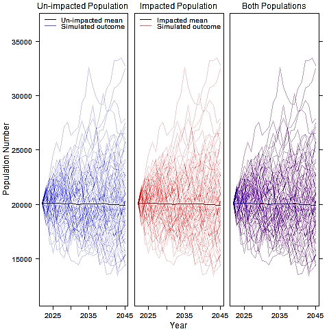
Figure 3.20: Minke Whale Scenario 4: Cumulative Projects, 1% Conversion Factor, no Vulnerable Subpopulation

3.4. Grey Seal

There appears to be negligible alteration to the growth trajectory of grey seal, regardless of which of the conversion factor scenarios were explored for the Proposed Development alone ( Figure 3.21 Open ▸ , Figure 3.22 Open ▸ , Figure 3.23 Open ▸ ). Comparison of the size of the unimpacted population to the impacted population for all three scenarios showed no difference in the number of animals with the median of the ratio predicted to be 100% at all time points and for all scenarios. Given these very small changes there is not considered to be a potential for long term effects on this species as the difference falls within the natural stochasticity of the modelled population.
Similarly for the cumulative scenario assessed within the north-east of Scotland no impacts were predicted on the population of grey seals, resulting from disturbance due to cumulative piling events ( Table 3.4 Open ▸ , Figure 3.24 Open ▸ ). This is not unexpected as both Seagreen 1A and Inchcape will finish piling prior to the commencement of piling at the Proposed Development so would not lead to a larger number of animals affected at any one time.

Table 3.4: Population Trajectory of Grey Seal Showing the Mean and Upper and Lower Confidence Limits at Different Time Points (Years After the Year in Which Piling Commences)

Figure 3.21: Grey Seal Scenario 1: 10% Reducing to 1% Conversion Factor, no Vulnerable Subpopulation

Figure 3.22: Grey Seal Scenario 2: 1% Constant Conversion Factor, no Vulnerable Subpopulation

Figure 3.23: Grey Seal Scenario 3: 4% Reducing to 0.5% Conversion Factor, no Vulnerable Subpopulation

Figure 3.24: Grey Seal Scenario 4: Cumulative Projects, 1% Conversion Factor, no Vulnerable Subpopulation

3.5. Harbour Seal

There appears to be negligible alteration to the growth trajectory of harbour seal, regardless of which of the conversion factor scenarios were explored. Comparison of the ratio of unimpacted population to the impacted population for all three scenarios showed no difference ( Table 3.5 Open ▸ ).
Results of the iPCoD modelling for harbour seal using the maximum adverse scenario 10% reducing to 1% scenario for the MU population (Scenario 1) show that the median of the ratio of the mean impacted population to the unimpacted population was one at four years (coinciding with the end of the first two piling campaigns) onwards until the maximum 25 year time point ( Table 3.5 Open ▸ , Figure 3.25 Open ▸ ). Therefore, there is not considered to be a potential for long-term effects on this species. These results were the same when using the 1% conversion factor scenario for the MU population (Scenario 2, Figure 3.26 Open ▸ ), and the 4% reducing to 0.5%conversion factor scenario for the MU population (Scenario 3, Figure 3.27 Open ▸ ), with the mean impacted population the same as the mean unimpacted population at time point 25. Since there is no discernible difference between the impacted and unimpacted populations there is therefore not considered to be a potential for any long-term effects on this species.
Similarly for the cumulative scenario assessed within the north-east of Scotland no impacts were predicted on the population resulting from disturbance due to cumulative piling events ( Table 3.5 Open ▸ , Figure 3.28:). This is not unexpected since both Seagreen 1A and Inchcape will finish piling prior to the commencement of piling at the Proposed Development so would not lead to a larger number of animals affected at any one time.

Table 3.5: Population Trajectory of Harbour Seal Showing the Mean and Upper and Lower Confidence Limits at Different Time Points (Years After the Year in Which Piling Commences)

Figure 3.25: Harbour Seal Scenario 1: 10% Reducing to 1% Conversion Factor, no Vulnerable Subpopulation

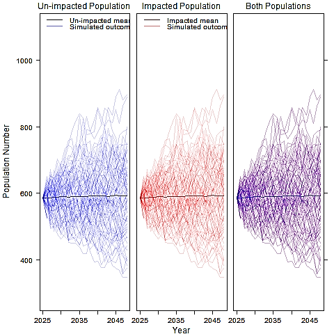
Figure 3.26: Harbour Seal Scenario 2: 1% Constant Conversion Factor, no Vulnerable Subpopulation

Figure 3.27: Harbour Seal Scenario 3: 4% Reducing to 0.5% Conversion Factor, no Vulnerable Subpopulation

Figure 3.28: Harbour Seal Scenario 4: Cumulative Projects, 1% Conversion Factor, no Vulnerable Subpopulation

4. Summary

This report presents the results of the iPCoD population modelling undertaken for key marine mammal species with the potential to be affected by the Proposed Development and for cumulative projects within relevant study areas. Overall, the iPCoD modelling results demonstrate that there is negligible significant effect to any species under any scenario assessed.
The population models were run to predict potential changes in population size as a result of piling at the wind turbine locations and offshore substation platforms associated with the Proposed Development. Reference populations were based on the latest estimates of population size for the relevant species’ Management Units. The numbers of animals disturbed were based on the maximum design scenario of a 4,000 kJ hammer energy only on the assumption that any population changes would be smaller considering the realistic hammer energy of 3,000 kJ which would affect smaller numbers of animals.
The modelling demonstrated that for all species there was predicted to be no long-term decline in the population with negligible to very small differences between the unimpacted to impacted population size. Even where there were notable differences in the number of animals within the undisturbed compared to the disturbed population (i.e. for minke whale using the 10% reducing to 1% conversion factor) it is considered likely that this variation will fall within the natural stochasticity of the population and therefore would not represent a measurable (and significant) difference.
Results were similar regardless of the conversion factor used to predict numbers of animals disturbed or assessed against a vulnerable subpopulation (harbour porpoise and minke whale). This suggests that even using the most conservative conversion factor of 10% reducing to 1%, the populations of all species are not predicted to be adversely affected by piling at the Proposed Development in the long term and are therefore likely to recover following cessation of piling. Furthermore, a precautionary assumption has been made for this study that animals are disturbed both on the day of piling and for 24 hours the following day leading to additional conservatism in the model.
Similarly, for cumulative projects where piling could occur sequentially and concurrently with the Proposed Development, there were no long-term population level effects predicted for any of the species. The assessment was based on the maximum design scenario for each respective cumulative project (i.e. largest number of animals potentially disturbed at any one time) and therefore represents a conservative approach to the cumulative assessment. Results should, however, be interpreted with caution as there were no details on the actual piling schedules for cumulative projects and it is likely that such activity would be phased due to global availability of piling vessels.
Though the iPCoD model attempts to model major sources of uncertainty, results will always vary greatly due to environmental and demographic stochasticity in the model (evidenced in the 95% confidence limits in population size; Table 3.1 Open ▸ to Table 3.5 Open ▸ ). Whilst the model shows no evidence of population change from the Proposed Development, there are sources of uncertainty. Variation in demographic rates among years may exist as a result of changes in environmental conditions, or as a result of random processes or chance events which impact vital rates (e.g. survival, fertility, etc.). In two, otherwise identical populations that experience exactly the same sequence of environmental conditions, demographic stochasticity will mean populations will follow slightly different trajectories over time. The model assumes that the effects of environmental variation on survival and fertility are adequately reflected by the range of values obtained from the expert elicitation (and shown in the spread of data around the mean trajectories Figure 3.1 Open ▸ to Figure 3.28:). In addition, the model assumes that survival and fertility rates are not affected by population size (i.e. that there is no density dependent response).
In summary, whilst it is understood that iPCoD is a relatively simple population model (which links days of disturbance to changes in individual vital rates), the most obvious sources of uncertainty have been captured in the model development. In addition, the marine mammal assessment has adopted a precautionary approach in recognition of the uncertainties in how animals respond to repeated piling over time.

5. References

Booth, C.G. and Heinis, F. (2018). Updating the Interim PCoD Model: Workshop Report - New transfer functions for the effects of permanent threshold shifts on vital rates in marine mammal species. Report Code SMRUC-UOA-2018-006, submitted to the University of Aberdeen and Department for Business, Energy and Industrial Strategy (BEIS), June 2018 (unpublished).

Booth, C.G, Heinis, F. and Harwood J. (2019). Updating the Interim PCoD Model: Workshop Report - New transfer functions for the effects of disturbance on vital rates in marine mammal species. Report Code SMRUC-BEI-2018-011, submitted to the Department for Business, Energy and Industrial Strategy (BEIS), February 2019 (unpublished).

Brandt, M. J., Diederichs, A., Betke, K. and Nehls, G. (2011). Responses of harbour porpoises to pile driving at the Horns Rev II offshore wind farm in the Danish North Sea. Marine Ecology Progress Series, 421, 205-216.

Carter, M. I. D., Boehme, L., Duck, C. D., Grecian, W. J., Hastie, G. D., McConnell, B. J., Miller, D. L., Morris, C. D., Moss, S. E. W., Thompson, D., Thompson, P. M. and Russell, D. J. F. (2020). Habitat-based predictions of at-sea distribution for grey and harbour seals in the British Isles. Sea Mammal Research Unit, University of St Andrews, Report to BEIS, OESEA-16-76/OESEA-17-78.

Czapanskiy, M. F., Savoca, M. S., Gough, W. T., Segre, P. S., Wisniewska, D. M., Cade, D. E. and Goldbogen, J. A. (2021). Modelling short‐term energetic costs of sonar disturbance to cetaceans using high‐resolution foraging data. Journal of Applied Ecology, 58(8), 1643-1657.

Donovan, C., Harwood J., King S., Booth C., Caneco B. and Walker C. (2016). Expert elicitation methods in quantifying the consequences of acoustic disturbance from offshore renewable energy developments. Pages 231-237. The Effects of Noise on Aquatic Life II. Springer.

Graham, I. M., Cheney, B., Hewitt, R., Cordes, L., Hastie, G. and Thompson, P.M. (2017). Strategic Regional Pre-Construction Marine Mammal Monitoring Programme 2017. Annual Report for the Moray Firth Regional Advisory Group.

Graham, I.M., Merchant, N.D., Farcas, A., Barton, T.R., Cheney, B., Bono, S. and Thompson, P.M (2019). Harbour porpoise responses to pile-driving diminish over time. Royal Society open science, 6(6), 190335.

Harwood, J., King, S., Schick, R., Donovan, C. and Booth, C. (2014). A protocol for implementing the interim population consequences of disturbance (PCoD) approach: quantifying and assessing the effects of UK offshore renewable energy developments on marine mammal populations. Report number SMRUL-TCE-2013-014. Scottish Marine and Freshwater Science, 5(2).

King, S. L., Schick R. S., Donovan C., Booth C. G., Burgman M., Thomas L., and Harwood J. (2015). An interim framework for assessing the population consequences of disturbance. Methods in Ecology and Evolution, 6, 1150-1158.

Sinclair, R.R., Sparling, C.E., and Harwood, J. (2020) Review of Demographic Parameters and Sensitivity Analysis to Inform Inputs and Outputs of Population Consequences of Disturbance Assessments for Marine Mammals. Scottish and Freshwater Science Vol 11 No 14. 78pp.

Sinclair, R., Booth, C., Harwood, J. and Sparling, C. (2019). Helpfile for the Interim PCoD v5 Model. March 2019.

Southall, B.L., Bowles, A.E., Ellison, W.T., Finneran, J.J., Gentry, R.L., Greene Jr, C.R., Kastak, D Miller, J.H., Nachtigall, P.E. and Richardson, W.J. (2007). Marine Mammal Noise-Exposure Criteria: Initial Scientific Recommendations. Aquatic Mammals 33 (4): 411–521.

Southall, B.L., Finneran, J.J., Reichmuth, C., Nachtigall, P.E., Ketten, D.R., Bowles, A.E. Ellison, W.T., Nowacek, D.P. and Tyack, P.L. (2019). Marine Mammal Noise Exposure Criteria: Updated Scientific Recommendations for Residual Hearing Effects. Aquatic Mammals 45 (2): 125–232.

Taylor, B.L. and DeMaster, D.P. (1993). Implications of non-linear density dependence. Marine Mammal Science, 9(4): 360 – 371.

[1] https://smruconsulting.com/?page_id=12050

[2] https://smruconsulting.com/?page_id=13194

[3] Note: Year 4 = Start of 2028 (After Completion of First Two Piling Campaigns) and Year 8 = Start of 2032 (After Completion of Third and Final Piling Campaign).