

1. Introduction
- This technical note provides information as requested by Marine Scotland Science (MSS) and NatureScot during the Berwick Bank Wind Farm Marine Mammals Road Map Meeting 2 (held on 20 October 2021) on the following topics:
- noise modelling methodologies which have been utilised on other offshore wind farm underwater noise assessments in the UK; and
- a review of energy conversion factors for determination of piling noise source sound exposure level (SEL).
2. Modelling Methodology
- Seiche Marine Technology Southwest (Seiche Ltd.) is a recognised expert in underwater acoustics that specialises in underwater acoustics and noise measurement. Seiche Ltd has supported renewables developers across the world comply with environmental regulations with respect to the effects of sound in water. Seiche Ltd. was commissioned by the Applicant to undertake and report the underwater noise modelling for the Berwick Bank Wind Farm that underpins the assessments reported within the EIA topic chapters.
- Seiche Ltd. proposes to utilise a robust, peer-reviewed noise propagation model for the Berwick Bank Wind Farm project in order to assess the effects of sound on marine life. In choosing the propagation model, it is important to ensure that it is applicable to the proposed development and surrounding area, including consideration of environmental variables, source types and frequency content etc.
- There are a number of models available for modelling of underwater noise propagation from a source. These include:
- ray-tracing (e.g. BOUNCE, BELLHOP);
- normal Modes (e.g. KRAKEN, KRAKENC);
- parabolic Equation (e.g. RAM, RAMS);
- fast-Field or Wavenumber Integration (e.g. SCOOTER, OASES);
- energy Flux (e.g. Weston Energy Flux model); and
- semi-empirical (e.g. Rogers, Marsh-Schulkin).
- The National Physical Laboratory (NPL) Review of Underwater Acoustic Propagation Models (Wang et al., 2014) provides a useful overview of many of these models and some of the pros and cons of using them in different situations, such as different water depths[1] and for different frequency ranges over which the calculation must be performed[2]. The suitability of some of the models is summarised in Table 2.1 Open ▸ .
Table 2.1: Suitability of Various Noise Models for Different Frequency Ranges and at Different Water Depths (Wang et al., 2014)
- MSS and NatureScot have requested details of underwater noise propagation models which have been used on previous offshore wind farm developments in the UK, along with a justification for the choice of noise model chosen for the Berwick Bank Wind Farm project. Seiche Ltd. has undertaken a review of publicly available offshore wind farm underwater noise assessment reports in order to provide this information to Marine Scotland (MS). This information is summarised in Table 2.2 Open ▸ .
- It should be noted that this review is based on information collated by Seiche Ltd., based on web-based searches and known projects. As such, it is likely that a number of additional offshore wind farm noise studies have been carried out and this review should not be considered a comprehensive or authoritative list.
- The consideration of the validity (or otherwise) for use of each noise model used on previous offshore wind farm studies for the Berwick Bank Wind Farm project is summarised in sections 2.2 to 2.4.
2.2. Weston Energy Flux Model
- Noise modelling studies were undertaken by the NPL for Greater Gabbard and Hornsea Offshore Wind One (HOW01). These studies utilise the Weston Energy Flux model (Weston, 1976; 1980a; 1980b). Some of the offshore wind farm noise modelling studies originally modelled by NPL using the Weston Energy Flux method were later updated by other consultancies. However, it is understood that the consultants who subsequently updated the noise modelling (e.g. in order to address changes in project design envelope, or to update the assessment in line with new injury and disturbance criteria) used their own methodology for the follow-on work. This is likely because the Weston Energy Flux model requires development of proprietary code in order to implement whereas other models are either available publicly (e.g. via the Acoustic Toolbox User interface and Post processor, AcTUP V2.2L) or already developed and available for use in-house.
- Despite requiring development of proprietary code, the Weston Energy Flux methodology is openly available through peer-reviewed publications and has been subjected to comparative studies in a number of peer reviewed-papers (e.g. Etter, 2013; Toso et al., 2014). According to the NPL noise modelling review report (Wang et al., 2014) the method is suitable across a wide range of frequencies in shallow waters. Given the Weston Energy Flux model’s known provenance and applicability, the water depth at the Berwick Bank Wind Farm (32.8 to 68.5 m) as well as its use in previous noise modelling studies for offshore wind farms in the UK, Seiche Ltd. has adopted this model as the primary noise modelling methodology for the Berwick Bank Wind Farm. In addition, Seiche Ltd. proposes to carry out a comparative calibration against other noise models (including the AcTUP based Parabolic Equation solver (RAMGeo), AcTUP based Normal Mode solver (KrakenC) and Rogers (1981) semi-empirical model) in order to ensure that the noise modelling outputs are robust and consistent.
2.3. Parabolic Equation Models
- The use of Parabolic Equation (PE) models for piling noise propagation modelling is well established in peer-reviewed literature as well as in practice, including for the Seagreen 1 and Neart na Gaoithe (NnG) offshore wind farms. One limitation of PE modelling is that the high computational requirements at higher frequencies means that it is typically limited to frequencies below 1 kHz (Wang et al., 2014). This means that use of the PE model alone can miss out the frequencies of most interest in assessing the effects of sound on high-frequency (HF) or very high-frequency (VHF) marine mammals when comparing against the NMFS (2018) and Southall et al. (2019) hearing-weighted SEL thresholds. Consequently, the model is often supplemented at higher frequencies by use of another model such as ray tracing, as was carried out for the NnG offshore wind farm. If assessment of HF and VHF cetaceans is an important outcome for the noise modelling assessment, then using PE modelling combined with another solver for higher frequencies is the more robust method (compared to using PE modelling alone). For this reason, Seiche Ltd. has utilised combined PE and ray tracing modelling on a number of occasions for sources including seismic source arrays and piling. However, the use of two different models can lead to discontinuities in the resultant attenuation terms where the two models meet, at the limits of their frequency validity. It is also significantly more time intensive to implement two separate models.
- For the Berwick Bank Wind Farm project, as discussed previously, Seiche Ltd. has chosen the Weston Energy Flux model which it is considered provides the most robust and consistent model for the frequencies and water depths of concern. However, it is proposed to use a PE model as part of the calibration of the Weston model to ensure that the noise model outputs are robust and consistent regardless of the choice of model.
2.4. INSPIRE
- The majority of UK offshore wind farm underwater noise studies accessed were modelled using the proprietary underwater noise propagation model “INSPIRE” developed in-house by Subacoustech ( Table 2.2 Open ▸ ). However, Seiche Ltd. has been unable to find any detailed information relating to the underlying noise modelling methodology adopted by INSPIRE. Nevertheless, based on a review of the various offshore wind farm reports, it is understood that the model takes into account:
- the geometrical spreading of sound from the source (based on a N log R relationship);
- the absorption of the sound by the seawater and sea-bed; and
- the bathymetry between the source and receiver positions.
- As such, it can be concluded that INSPIRE is a semi-empirical model based on basic propagation concepts, although it is understood that there is some form of calibration built in (no evidence or calibration results could be found in the public domain). It is therefore not possible to comment on the validity or otherwise of the model for any of the developments for which it was utilised. Likewise, taking into consideration that INSPIRE is not publicly available, not peer reviewed, is of unknown provenance and cannot be independently verified in terms of its applicability, it is concluded that this noise model is unlikely to be suitable for use by Seiche Ltd. on the Berwick Bank Wind Farm project.
- It is worth noting that the INSPIRE model also incorporates a black-box approach to prediction of the pile source level which, likewise, is of unknown provenance.
Table 2.2: Review of Noise Modelling Methodology used for Previous OWF Developments
3. Pile Source Noise Determination
3.1. Summary of General Concepts
- The sound generated and radiated by a pile as it is driven into the ground is complex, due to the many components which make up the generation and radiation mechanisms. Larger pile sizes can require a higher energy in order to drive them into the seabed, and different seabed and underlying substrate types can require the use of different installation techniques including varying the hammer energies and the number of hammer strikes. In addition, the seabed characteristics can affect how ground-borne noise propagates from the pile, thus fundamentally affecting the acoustic field around the activity. The type of hammer used can also affect the sound characteristics. For example, use of a longer duration hammer strike (in relation to the impulse shape) can result in significant reductions to the sound emissions from piling (Nehls et al., 2007). Likewise, the BLUE hammer technology uses a combustion chamber and water column to significantly reduce the impulsivity of the strike with significant reduction to the noise characteristics, compared to steel hammers. As a result, there can be significant variation in the sound radiated into the water column depending on the various different parameters particular to a site.
- Underwater noise sources are usually quantified using a decibel (dB) scale with values generally referenced to 1 μPa pressure amplitude as if measured at a distance of 1 m from a hypothetical, infinitesimally small source (called the Source Level). This quantity is often referred to in the literature as an equivalent monopole source level. In practice, it is not usually possible to measure at 1 m from a source, but the metric allows comparison and reporting of different source levels on a like-for-like basis. In reality, for a large sound source such as a pile, this imagined point at 1 m from the (theoretical, infinitesimally small) acoustic centre does not exist. Furthermore, the energy is distributed across the source and does not all emanate from this imagined acoustic centre point. Therefore, the stated sound pressure level at 1 m does not occur at any point in space for these large sources. In the acoustic near field (i.e. close to the source), the sound pressure level will be significantly lower than the value predicted by the Source Level.
- A useful measure of sound used in underwater acoustics is the Sound Exposure Level, or SEL. This descriptor is used as a measure of the total sound energy of an event or a number of events (e.g. over the course of a day) and is normalised to one second. This allows the total acoustic energy contained in events lasting a different amount of time to be compared on a like for like basis. The SEL is defined as:
|
| Equation 1 |

- where
 is the integration time of the sound “event”,
  is the squared sound pressure at a time
  and
and  is the reference time-integrated squared sound pressure of 1 µPa2s. For impulsive sounds it has become customary to utilise the T90 time period for calculating and reporting Root-mean sound pressure levels (RMS). This is the interval over which the cumulative energy curve rises from 5% to 95% of the total energy and therefore contains 90% of the sound energy.
 - Based on this definition of SEL, and assuming a point source, the total acoustic energy (H) radiating into the water can be written as:
|
| Equation 2 |
- where
 is the characteristic impedance of seawater (De Jong and Ainslie, 2008). In this equation, the value 120 in the exponent bracket represents the reference time-integrated squared sound pressure (i.e. 20 log 1 x 10-6 = 120).
 - It is possible to determine the ratio of the hammer strike energy to sound energy which is radiated into the water (also referred to as Energy Conversion Factor, β) by dividing the sound energy (H) by the hammer energy (E).
|
| Equation 3 |
- By rearranging the above formulas, it is possible to state the source SEL in terms of the hammer energy (E) and energy conversion factor (β) as follows
|
| Equation 4 |
- Consequently, if the energy conversion factor can be estimated for any given pile, it is possible to estimate the source SEL based on the hammer energy used to install the pile. More detailed consideration of the energy conversion factor and its implications for noise modelling are presented in the following sections.
3.2. Determination of Source SEL from Measurement Data (Extrapolation)
- The equivalent source monopole SEL is not a directly measurable quantity. It is therefore usually necessary to determine the source SEL from piling by extrapolating a line of best fit through measurements undertaken at some distance (usually several hundred metres or more) back to a distance of 1 m from the pile’s theoretical central point. This is often done by fitting a curve through the measured data using a N log R + αR relationship[3], where R is range, N represents the geometrical divergence slope and α represents an empirically derived correction for energy loss (e.g. molecular absorption of acoustic energy etc.). This methodology is widely used but is rudimentary. Consequently, wide scale errors can (and do) occur in determination of source SEL based on even small differences in propagation coefficients which are based on more distant measurements.
- An illustrative example of how the line of best fit through data can affect the apparent source level is presented in Figure 3.1. For this hypothetical example, the green crosses (location X) are higher in magnitude than the red diamonds (location Y) at locations further from the pile (10 km), but similar in magnitude closer to the pile at distances of up to 2 km. However, variations in sound levels measured at the greater range of 10 km result in a different slope and intercept. In this illustrative example, relatively small variations in the 10 km SELs (typically 5 dB) result in a difference of 15 dB in the apparent source SEL. However, given that the closer “measurements” are of a similar magnitude, this would likely be as a result of variations in propagation further from the source, such as due to changes in bathymetry or bottom sediments, geology and sound speed gradient, or due to uncertainty and variability in the more distant measurement data. Another important point to note is that the location X values at larger ranges are actually higher than location Y, even though the derived source SEL is significantly lower.

Figure 3.1: Hypothetical Example Showing How a Small Variation in Propagation at Large Ranges Can Significantly Affect the Derived Source SEL when Using Extrapolation
- It is worth noting that the illustrative example in Figure 3.1 was based on hypothetical noise modelling with a source SEL input of 210 dB re 1 µPa2s for both scenarios. The model was run for two scenarios: each using different sediment geoacoustic parameters and bathymetry profiles in order to simulate variability in received SEL values at larger ranges.
- The source SEL for the model was derived based on a 1% energy conversion factor for an 800 kJ hammer (i.e. a source level of 210 dB re 1 µPa2s). The source level of 224 dB re 1 µPa2s which was derived by extrapolation for Location Y would result in an apparent energy conversion factor of 14%, which is fourteen times higher than the known[4] energy conversion factor used as an input to the model. Again, it is important to reiterate that the lower received SEL values resulted in the higher derived source SEL and energy conversion factor. It follows that, since the large-scale errors in determination in source SEL are introduced by additional absorption of sound energy at larger ranges, these errors are likely to result in an overestimate. Consequently, particular caution should be used for any source SELs or energy conversion factors which are unusually high compared to other similar measurements, based on large propagation ranges or higher than would be expected based on scientific and theoretical considerations. It should be noted that large errors in extrapolation could still be encountered if full acoustic modelling is used, particularly where there are uncertainties in the input parameters such as bottom and surface conditions, bathymetry and sound speed profile outside of the measurement range. Such errors are likely to be larger at greater ranges from the pile and therefore measurements conducted close to the pile are likely to result in more robust estimates of source level and conversion factor than more distant measurements. Furthermore, there will always be some error introduced into any source derivation caused by variations in received SELs due to measurement uncertainty.
- It is also worth noting that the higher derivation of source SEL would only be appropriate if this value was used as an input to a model which used the same or similar propagation terms as were used in the extrapolation. However, even if such a model was constructed it is likely that predicted noise levels at distances closer to the source than the nearest measurement point would be overestimated.
- In summary, interpolation and extrapolation of measured noise data is only acceptably accurate as long as the data is not extrapolated significantly beyond the range of the measured data. By definition, this means that this method is not well suited to determining an equivalent monopole source level at 1 m. An alternative method of determining the source SEL is to undertake full acoustic modelling, which is preferable to the extrapolation method in that it can, to some extent, account for acoustic effects outside the measurement data range. In general, studies which utilise a full acoustic model (such as parabolic equation or Weston energy flux) will provide more reliable estimates and greater weight should be placed on the results of such studies, although some caution still needs to be observed particularly if the model input parameters are not very well defined outside of the measurement range. Even where full acoustic modelling is used, it is still likely that small differences in attenuation terms could lead to widescale overestimates of the source SEL and conversion factor if the study is based on more distant measurements (e.g. >300 m) due to differences in real world propagation and the model assumptions.
- Based on the considerations discussed above, it is concluded that:
- Any source SEL or energy conversion factor derived from measurement data needs to be interpreted very carefully and cannot be blankly accepted or adopted as if it is a directly measurable quantity.
- Energy conversion factors might only be applicable for use in an acoustic model which uses similar propagation terms to those for which it was derived.
- Particular care needs to be taken when using energy conversion factors based on more distant measurements.
- Use of extrapolation at larger ranges will tend to overestimate the source SEL at 1 m and therefore result in a significant overestimate of the energy conversion factor.
- Greater weight should be placed on studies which utilise full acoustic modelling as opposed to extrapolation of measured data significantly beyond the range of that data using a N log R fit or similar. In either case, it is important to understand that the source SEL and derived energy conversion factor are estimates based on the model used and subject to potential wide-scale errors and uncertainty.
- In general, estimates of source level based on more distant measurements (e.g. >300 m) will result in potentially widescale errors in determination of the pile monopole source SEL and energy conversion factor, even in studies using full acoustic modelling.
3.3. Review of Energy Conversion Factors in Literature
3.3.1. Studies Based on Theoretical Considerations
- Use of an energy conversion factor allows the source SEL of piling to be estimated based on a given hammer strike energy. This is desirable because it allows different piling scenarios to be modelled including the effects of soft-start, energy ramp-up and use of different hammer energies for different pile types and sizes and for different ground conditions (e.g. use of higher hammer energy in harder ground). If this approach is used, it is therefore necessary to derive a robust estimate of the energy conversion factor to avoid overestimating or underestimating the potential impact.
- A detailed numerical study of the sound generating mechanism of impact pile driving is set out in Zampolli et al. (2013). Based on the results of theoretical assumptions and calibration against measured noise from piling, the paper estimates that the ratio between the energy transferred into the water and the energy which is transferred into the pile from the hammer is 0.0213 (2.13%). It is important to understand that the energy transferred from the hammer into the pile (which was reported as 54.6 kJ) is not the same as the hammer energy (which was reported as 87 kJ). Accounting for losses and inefficiencies in the transfer of energy from the hammer to the pile the energy conversion factor between the hammer energy and radiated acoustic energy will be lower.
- A study by Flynn and McCabe (2019) shows measured real world hammer efficiencies of between 15% and 70% with a strong linear relationship with hammer energy (drop height). For hydraulic hammers, there is a greater efficiency of energy transfer when it is working towards the upper end of its rated energy. Consequently, for a typical piling scenario consisting of soft start followed by low power piling followed by a ramp up to a higher energy followed by full pile piling only at the end of the sequence, it is likely that energy transfer efficiencies will be at the lower end of this scale for the majority of the pile installation. For a 15% hammer energy efficiency this equates to an energy conversion factor between the hammer energy and radiated acoustic energy of β ≈ 0.3% whereas a 70% hammer energy efficiency equates to β ≈ 1.5% for full power piling.
- Using the reported hammer energy of 87 kJ for the Zampolli et al. (2013) study, the energy conversion factor can be calculated to be β ≈ 1.3%, which is within the range predicted by theoretical considerations of hammer energy transfer.
3.3.2. Energy Conversion Factors based on Measurements in Published Literature
- Energy conversion factors have been reported for full scale observational studies in a number of publications.
- Robinson et al. (2007) undertook controlled measurements on a pile utilising an 800 kJ hammer and a range of hammer energies (where the hammer energy was gradually increased from 10% to 100% of the full energy level). The study concluded that the energy conversion factor between hammer energy and energy radiated into the water column is β ≈ 0.3% based on the observed data over the full range of hammer energies. The study also concluded that the approximately linear relationship between the hammer energy and SEL demonstrates that it is possible to extrapolate to higher hammer energies with reasonable accuracy. A similar linear relationship has been reported in a number of other studies (e.g. Bailey et al., 2010; Robinson et al., 2007; Robinson et al., 2009; Lepper et al., 2012; Robinson, Theobald, and Lepper, 2013).
- Measurements by De Jong and Ainslie (2008) for the Q7 wind farm on 4 m diameter piles using an 800 kJ hammer determined that the total acoustic energy radiated into the water column was approximately β ≈ 0.8% of the hammer energy. The study notes that the distance of the measurements used in the study (1 km from the pile) was too large to derive a reliable estimate of source SEL and referred to the Robinson et al. (2007) study which took measurements much closer to the pile (57 m). Interestingly, both studies measured similar received levels at comparable ranges. It is therefore concluded that the β ≈ 0.8% energy conversion factor found by De Jong and Ainslie (2008) was likely an overestimate and that the Robinson et al. (2007) study, using closer measurements to the pile, provides a more robust estimate of source SEL and energy conversion factor.
- Dahl and Reinhall (2013) carried out a detailed study using beamforming from a vertical hydrophone array which concluded that β ≈ 1%. This study was based on 0.762 m diameter piles using a 180 kJ hammer. Dahl et al. (2015) concluded that β ≈ 0.5% was a representative factor, based on a review of the Robinson et al. (2007), Dahl and Reinhall (2013) and Zampolli et al. (2013) papers.
- One study for Beatrice Offshore Windfarm Limited (BOWL) using a submersible impact hammer on pin piles found an energy conversion factor of between β ≈ 1% and β ≈ 10% (depending on pile penetration) (Thompson et al., 2020). The higher conversion factors were found for longer exposed lengths of pile towards the start of the piling and reduced to 1% as the pile penetrated further into the seabed. In contrast to the more traditional piling method where the impact hammer remains above water (or remains above water for a large proportion of the piling sequence), this was for a method of installing piles where the pile is driven using a submersible hammer starting just above the water surface and ends up with an exposed length only 2 m above the seabed in water depths of 35 to 45 m. The results of this study showed that for submersible hammer piling the source SEL depended on a combination of the hammer energy and exposed pile length above the seabed.
- It is important to note that for the BOWL study the pile does not penetrate above the water line (or if it does this does not occur for more than the first few strikes) and therefore the length of pile exposed to the water reduces as the pile penetrates. Consequently, the surface area which can radiate sound into the water reduces as the pile penetrates into the seabed resulting in the reduced source SEL levels as piling progresses. With the traditional (above water) piling the pile is exposed above water at the end of the piling sequence, meaning that the length of pile exposed to the water remains the same throughout. Consequently, radiated noise from piles installed using above water hammers is characterised by noise levels typically increasing as the pile penetrates the seabed. This is due to increasing hammer energies being required to drive the pile as the soil resistance increases with depth of penetration. This is corroborated by the majority of piling noise measurements in the literature which clearly demonstrate a strong dependence on hammer energy.
- A more detailed study of the acoustics of submersible pile hammers is provided in Lippert et al. (2017) which compares detailed numerical modelling of submersible pile driving with measured data. This study included measurements and detailed source modelling for four skirt piles with an outside diameter of 2.44 m and a length of 82 m, which were driven into the sandy seabed through the jacket structure, in water depths of 40 m. Each of the piles was driven to a final penetration of 65 m below seabed.
- According to Lippert et al. (2017) the source level of the pile is approximately proportional to both the hammer energy and, once the pile is below the water line, the length of pile exposed. The study found that the highest sound levels are typically encountered at the point when the pile is approximately flush with the sea surface (i.e. has already penetrated by some distance from above the water line) and then reduces by approximately 2.5 dB per halving of exposed length once below the surface. Seiche Ltd. has carried out further analysis of the Lippert et al. (2017) data in order to derive a conversion factor for the piling sequence, as shown in Figure 3.2. Seiche Ltd. converted the reported broadband source SEL into total acoustic energy (H) using equation 2, and the conversion factor (β) was determined using equation 3 and the normalised pile hammer energy (E).
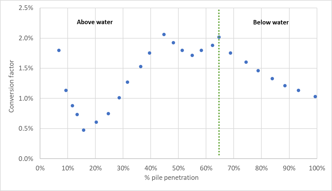
Figure 3.2: Analysis of the Relationship Between Conversion Factor and Pile Penetration for a Submersible Hammer Based on Data from Lippert et al. (2017)
- The Lippert et al. (2017) study also notes that there is a brief period at the start of piling where the source sound level strongly decreases over the first few meters of penetration caused by the change in pile‐soil interaction. These are important aspects to consider for the Thompson et al. (2020) study where piling started with the pile at this most critical location in terms of noise emissions and this needs to be factored into any understanding of the applicability or otherwise of the piling noise characteristics. In other words, the piling for the BOWL foundations suffered from a combination of factors at the start of piling which are unlikely to occur in situations other than where the pile hammering commences when the pile head is approximately flush with the water surface.
- It is a well established principal that the size of the pile being installed will affect the way that sound is radiated into the water (e.g. Nehls et al., 2007). For a given blow energy, when the pile diameter increases, the radiating surface increases, but as long as the pile driver energy is not raised the amplitude decreases. This is because the available exciting force has to excite a larger number of surface elements. Hence a larger diameter for any given hammer energy is more likely to produce lower sound levels than for a smaller diameter with the same energy (Nehls et al., 2007). It is therefore likely that larger piles will result in a lower energy conversion factor than for installation of smaller piles of the same energy. This provides additional difficulties with regards to the application of energy conversion factors from studies on smaller pin piles (such as those in the Thompson et al., 2020 study of up to 2.2 m diameter) to installation of large piles (such as those proposed for the Berwick Bank Wind Farm which are up to 5.5 m diameter).
- Seiche Ltd. has contacted the primary author of the BOWL study , who has expressed concern with respect to the validity of adopting the results from the BOWL study to different piling techniques or to different sites (i.e. other than the specific case of applying the conversion factors to the site and model used at BOWL) (Prof. P. Thompson, University of Aberdeen, pers. comm.).
- Notwithstanding the question of the validity of using the study findings at other sites or as a proxy for different piling techniques, there a number of concerns about applying the derived energy conversion factors from the study to any other study, whether using a submersible hammer, above water hammer, pin piles or monopiles. The methodology used to derive the source levels and conversion factors in the study can be summarised as follows:
- Use acoustic model to predict the expected broadband transmission loss each monitoring location based on generic piling spectrum shape.
- Add the modelled broadband transmission loss value at each location to the measured broadband SEL in order to derive the apparent source SEL.
- Use the derived source SEL and logged hammer energy to determine the apparent energy conversion factor.
- The inherent assumption in the above methodology is that the modelled broadband transmission loss can be added to the measured SEL (which might have a different spectrum shape) in order to accurately determine the source SEL. However, given that the measurements used in the analysis were all taken at a relatively large range for the pile (between 770 m and 11 km) it is likely that potentially significant differences could occur between the modelled and real world transmission loss. It is also noted that the noise modelling undertaken does not account for the change in source location as the pile penetrates the substrate. What starts off as a line source generating a Mach wave throughout the entire length of the water column becomes a much smaller source and constrained to a lower part of the water column as piling progresses. If the modelling did not take this into account, then this could result in further errors in determining the source SEL and energy conversion factor.
- To investigate potential differences between the modelled transmission loss and real-world transmission loss further, Seiche Ltd. has undertaken a more detailed analysis of the raw data provided as supporting information for the study. Inspection of the data shows a strong variation in the derived source SEL depending on the location of the monitor for any given blow. For example, pile B2 at turbine F13 shows significant variation for the same blow number (blow 10) which has a conversion factor of 6% or 13% depending on which measurement location is used. For turbine F13, pile B2, blow 11 the analysis likewise results in a conversion factor of 5% and 12% for the same blow depending on which measurement point is analysed. This same pattern where the conversion factor is dependent on measurement range is apparent throughout the dataset, demonstrating that the quoted conversion factor is as much if not more an indication of differences between the model and real-world propagation as it is of acoustic energy emitted into the water.
- To progress this analysis further, Seiche Ltd. has plotted the difference between measured and modelled SEL against range in Figure 3.3. The results show higher differences between the measured and modelled SELs at larger ranges compared to the closer measurements which is strongly indicative of errors in the modelling compared to real world propagation. The analysis shows that the differences are smaller closer to the pile and, therefore, the method used would determine a lower source level (and therefore lower conversion factor) using closer data. As an example, the difference of 3 dB in the mean values between using the “all data” dataset (i.e. the data used for the analysis presented in the Thompson et al., 2020 paper) and data at distances of less than 1 km would result in a halving of the average energy conversion factors (i.e. 5% rather than 10%). In other words, the apparent energy conversion factors found in the study are a manifestation of differences between the modelled transmission loss versus real world transmission loss rather than a measure of the true acoustic energy radiated into the water by the pile.

Figure 3.3: Analysis of the Relationship between Distance and the Difference between the Modelled and Measured SEL for BOWL Piling Based on Raw Data from Thompson et al. (2020)
- It should be noted that whilst the trend shown in Figure 3.3 can be seen when looking at data from all piles (which is the way that the data was analysed in the Thompson et al., 2020 study) the picture becomes more complex when investigating individual pile measurements within the data set. For many piles (e.g. pile F11-A2 as shown in the left of Figure 3.4) there is a significant difference between the conversion factors calculated based on different measurement positions. In the case of this pile (F11-A2), measurements at ∼4 km resulted in significantly higher conversion factor estimates than measurements at ∼11 km. In other cases (e.g. pile G13-A1 in the lower half of Figure 3.4) there is much closer correlation between datasets which is based on measurements at <1 km and ∼11 km. For some reason, most likely due to a characteristic of the noise modelling, the results at ∼4 km tend to result in a significantly higher conversion factor for the majority of piles, compared to measurements at circa 1 km, 2 km or 11 km (which reflects the overall trend seen in Figure 3.3). In this respect the data definitively highlights the problematic nature of quoting conversion factors derived from the study as if they are a “real” quantity (whilst at the same time it is important to note that the amount of sound radiated into the water is not dependent on the measurement range). In any case, the fact that the measurements which show the closest correlation between different measurement ranges (i.e. pile G13-A1 in the lower half of Figure 3.4) also show lower conversion factors leads to the likely conclusion that the conversion factors quoted from the study are overestimated.
|

Figure 3.4: Conversion Factors Derived for Two Different Piles (F11-A2 Using Measurement Data at ∼4 km and ∼11 km and G13-A1 Using Measurement Data at <1 km and ∼11 km) Based on Raw Data from Thompson et al. (2020)
- It is notable (and regrettable) that all of the closer measurements to the pile (<780 m) overloaded and could not therefore be used in the analysis since it is likely that this would have demonstrated even smaller differences between modelled and measured levels and it follows that these would have provided a much better indication of the source SEL. Using this closer measurement data set is likely to have found that the energy conversion was significantly lower than reported in the paper and even lower than, for example, the ∼5% figure derived by reanalysing the data at <1 km.
- It is therefore concluded that the source SEL and conversion factors reported in Thompson et al. (2020) are not a measure of “real” conversion factors, but are a reflection of differences between measured data and the noise modelling. The quoted conversion factors are likely to be a gross overestimate of the amount of energy radiated into the water and should not form the basis of source level estimations for other studies. Furthermore, the methodology and assumptions used in the study mean that even if the conversion factors could be corrected or estimated based on a reanalysis of the raw data, it is unlikely that the findings would be directly applicable to other sites or situations.
- Nevertheless, the study (along with the robust modelling and measurements set out in Lippert et al., 2017) provides a useful indication of how noise from piling using a submersible pile hammer varies depending on pile penetration depth.
3.3.3. Review of Measured UK OWF Piling Noise Data
- In order to supplement the published literature on energy conversion factors, Seiche Ltd. has undertaken a review of publicly available noise measurements for offshore wind farm construction on the marine data exchange website. This review only includes the measurements for which the report authors included an estimate of the source SEL as well as details of the hammer energies used. The source SELs in many of the reports were based on an extrapolation of measured data using a line of best fit between data points. As such, the source SELs in the reports are potentially significantly affected by variations in propagation characteristics at each site and it is important that caution is used when using these values in any analysis.
- It is noted that a large number of the uploaded reports did not report the SEL metric (or the source SEL) and instead report only peak-to-peak and the now depreciated dBht metrics. Consequently, a large number of monitoring studies could not be included in the review.
- In order to determine the energy conversion factor, Seiche Ltd. converted the reported broadband source SEL into total acoustic energy (H) using equation 2, and the conversion factor (β) was determined using equation 3 and the reported pile hammer energy (E). The results of the review are shown in Table 3.1 Open ▸ .
Table 3.1: Review of UK Offshore Wind Farm Source SELs and Hammer Energies
- As discussed previously in this report, it is important to understand that the source SEL level is not a directly measurable quantity. Wide scale errors can (and do) occur in determination of source SEL based on even small differences in propagation coefficients, especially those which are based on more distant measurements.
- Many of the studies estimated widely different source SEL levels based on measurements of very similar received levels at short to medium ranges (e.g. 100 m to 500 m). Where there were widely different source estimates these are considered to be primarily due to variations in propagation at larger ranges from the pile and widescale errors introduced by extrapolating data well beyond the measurement range. One such example is Greater Gabbard where a high reported source level of 223 dB re 1 µPa2s for pile IGJ02 was some 24 dB higher than the source level reported for pile IGH03. However, inspection of the data shows that the measured SEL at ranges of 100 m to 750 m differed by only 2 to 4 dB. The significantly higher source level at pile IGJ02 was therefore an artifact of the propagation coefficients (e.g. 18 log R for IGJ02 vs 9.5 log R for IGH03) which led to a wide variation in source SEL and therefore significant variations in the apparent energy conversion factors. This is an excellent example of the issues with reporting SEL source levels based on extrapolated data and how it is important to exercise caution when interpreting quoted source SELs and conversion factors. To be clear, the quoted source level of 223 dB re 1 µPa2s for pile IGK02 in this study can only be considered an accurate estimate if it is used in noise modelling which uses the same propagation method and associated coefficients as were used to derive the source SEL, and even then only within the measurement range itself. Using this source level in a full acoustic model (or any other model) would lead to widescale errors and the derived energy conversion factor of 20% is therefore highly misleading and little weight should be attached to this number.
- A similar effect can be seen in the data for Sheringham Shoal OWF where the highest source SEL and conversion factor (pile G6) resulted in a lower received SEL at 500 m than the lowest source SEL and conversion factor (pile I4). Again, the higher source level (and subsequent energy conversion factor derived from those measurements) was an artifact of the propagation terms derived using more distant measurements, and was therefore more a reflection of distant propagation than the source energy per se. A similar effect can be seen in the Rampion noise monitoring data where the derived source SEL (and the energy conversions derived from them) based on more distant measurements of received SEL resulted in a higher derivation of source level. Likewise, measurements at Teeside OWF show highly unusual propagation conditions (e.g. a 6 dB difference between the derived SEL at 500 m and 750 m) which would also result in potentially largescale errors in the determination of source SEL.
- Another important factor to consider when interpreting results is whether the quoted source SELs (and therefore the derived energy conversion factors) are based on percentile, average or maximum received levels. Some of the reports reviewed (e.g. Teeside OWF) used the maximum received levels in order to derive the source SEL. Given the large variation in received sound levels, especially at larger ranges from the pile, this could lead to a widescale overestimate of the average or typical energy conversion factors.
- In conclusion, it is important to understand that the studies reviewed in this section were undertaken for the primary purpose of complying with permit conditions on monitoring and were not designed to provide robust estimates of the source SEL or conversion factor. Indeed, none of the reports mentioned or attempted to derive a conversion factor as part of the analysis. The significant range of derived source SELs in the studies is not typically reflected by the measured data at more distant measurement locations and potentially gross errors and uncertainties in the derivation of source SEL are therefore concluded to be too great to form any consensus view on a conversion factor.
3.3.4. Conclusions on Energy Conversion Factor and Application to Berwick Bank Wind Farm
- Taking the above analysis into account, it is important to understand that the source SEL is a theoretical construct which is useful in noise modelling to estimate the SEL in the far-field. In general, higher source SELs found in the various reports, and the conversion factors derived from them, are associated with (and indeed caused by) higher propagation coefficients as a result of extrapolating measurement data well beyond the measurement range, or simply due to errors introduced by measurements at larger ranges. Taking this into account, it is difficult to determine a preferred site or receiver location independent energy conversion factor for use in modelling a wide range of scenarios. Nevertheless, it is considered that greater emphasis should be placed on peer reviewed studies, theoretical scientific considerations and studies which utilise full acoustic modelling to determine the source SEL since these are less prone to errors introduced by extrapolating measured data beyond its range of validity.
- Given the higher conversion factors are generally significantly affected by long range propagation factors, it is considered that use of these higher numbers could lead to significant overprediction of the far-field sound levels when using propagation models which do not correspond to the propagation coefficients used in the determination of the source SEL in the first place. High source SELs and energy conversion factors derived from these would only be appropriate if used in the same model as was used to derive the source level. In this respect, it is important to take into account that the Berwick Bank Wind Farm will be modelled using a full acoustic model (as opposed to a N log R relationship).
- Based on the peer reviewed literature which considers theoretical concepts, and is therefore less prone to measurement uncertainty, it is concluded that a representative energy conversion factor using an above water hammer is likely to be in the range β ≈ 0.3% to 1.5% (Zampolli et al., 2013), whereas Dahl et al. (2015) concluded that β ≈ 0.5% based on a review of both theoretical considerations and measurement data by others. The theoretical upper limit of the energy conversion factor is therefore approximately 1.5%, although this is only likely to apply when the hammer is operating at the very top end of its power rating (maximum drop height), with lower efficiencies being more likely throughout the majority of the piling period (and importantly when the marine mammal is closer to the pile). It is therefore concluded that a hammer energy conversion factor of β ≈ 1% is a representative and precautionary value across the range of hammer energies used during a pile installation. Nevertheless, it is important to note that this is a potentially over-precautionary estimate and that the current scientific consensus is that the typical conversion factor is β ≈ 0.5%.
- Peer reviewed studies based on empirical measurements on above water piling hammers determined real world energy conversion factors of β = 0.3% (Robinson et al., 2007), β = 0.8% (De Jong and Ainslie, 2008) and β ≈ 1% (Dahl and Reinhall, 2013). The larger of these three numbers (β ≈ 1%) is consistent with the 1% average hammer energy conversion factor based on the theoretical considerations. Taking into account the various factors discussed previously, including importantly the effect of large propagation ranges on source determination and errors in extrapolation, it is concluded that the measured data from UK offshore wind farms generally supports this conclusion.
- However, it is recognised that use of a submersible hammer can result in the conversion factor varying depending on pile penetration depth. Both measurement data and detailed source modelling presented for a partially submersible hammer in Lippert et al. (2017) supports a varying conversion factor of between β ≈ 2% and 0.5% depending on penetration depth and the length of pile above water. Thompson et al. (2020) whilst ostensibly indicating conversion factors ranging between β ≈ 10% and 1% for a fully submersible hammer is considered to be a gross overestimate of the true energy radiated into the water caused by discrepancies between the noise modelling and real world propagation. True conversion factors (i.e. in relation to the total acoustic energy radiated into the water column) are thought likely to be in the order of half these values, or less. Of the two studies, the Lippert et al. (2017) study is considered more scientifically robust because of the very strong correlation between the detailed finite element modelling and measured data, compared to the Thompson et al. (2020) study where the conversion factors are a reflection of the discrepancy between measured data and modelled data.
- Nevertheless, it is recognised that for the Lippert et al. (2017) study a significant proportion of the pile was above water at the start of the piling sequence which could have reduced the apparent conversion factor compared to a situation where the pile starts just above the water line. The 82 m length piles were driven to approximately 17 m above the seafloor in 40 m water depth for the Lippert et al. (2017) study. Assuming that the energy radiated into the water is approximately proportional to the length of pile which is exposed to the water then the conversion factor at the start of piling in the Lippert et al. (2017) study can be estimated to be approximately 3.5% had the water been deeper (i.e. approximately 80 m deep, such that the pile just penetrated above the water line at the start of piling). For the Berwick Bank Wind Farm, although no detailed piling methodology is available at this point in time, it is likely that in the deepest waters the piles will start off just above (or just below) the water line, ending up penetrating just above the seafloor in water depths of up to 68.5 m. Consequently, and in light of Marine Scotland Science and NatureScot’s request to use a conversion factor of 4% at the start of piling, a conversion factor of β ≈ 4% has been used for the Berwick Bank Wind Farm at the start of the piling sequence. This 4% conversion factor is higher than that derived in the Lippert et al. (2017) study and is therefore considered conservative. Furthermore, it should be noted that any piles installed in shallower waters within the Berwick Bank Wind Farm are likely to result in lower source levels than derived for the start of piling here because a significant proportion of the pile could penetrate above the water line, meaning much of the energy would radiate into the air rather than water.
- In the Lippert et al. (2017) study the piles remained approximately 17 m above the seafloor (i.e. 42.5% of the water depth) at the end of piling which, using the same logic, means that the β ≈ 1% conversion factor at the end of the piling sequence is likely to be an overestimate compared to the Berwick Bank Wind Farm case where a greater proportion of the pile will penetrate the seabed. Since the final pile position in the Lippert et al. (2017) study was a little below mid-water depth (and since, when the pile is subsea, the falloff in acoustic energy cited by Lippert et al. (2017) is ~2.5 dB per halving of exposed pile above the seabed), a final conversion factor of 0.5% or less at the end of piling can be inferred.
- Consequently, based on this review, the assumption that piling is likely to use a submersible hammer, best available scientific evidence, professional judgement, and taking into account the advice of Marine Scotland Science and NatureScot, it is proposed to utilise a varying energy conversion factor of β = 4% at the start of piling to 0.5% at the end of piling for noise modelling at the Berwick Bank Wind Farm. However, in light of potential uncertainties in the derivation of source level it is also proposed to carry out a sensitivity analysis using a conversion factor of β = 10% at the start of piling to 1% at the end of piling as well as a scenario utilising a conversion factor of 1% throughout the piling sequence for comparison purposes. The latter conversion factor of 1% throughout is considered representative of a scenario where above-water hammers are used, although it is considered unlikely to be the case at the Berwick Bank Wind Farm.