

3. Results
3.1. Harbour Porpoise
- Results of the iPCoD modelling for harbour porpoise using the maximum adverse design of 10% reducing to 1% conversion factor for the MU population (Scenario 1) are presented in Table 3.1 Open ▸ and Figure 3.1 Open ▸ . Results are expressed as the predicted difference in the mean population size of an undisturbed population versus a disturbed population and is provided as the median of the ratio of impacted to unimpacted population size (also referred to as the ‘median counterfactual of population size’; Sinclair et al., 2020). Thus, for a ratio of one there is no difference between the trajectories of disturbed versus undisturbed populations. Conversely, for a ratio of <1 the median impacted population size is smaller than the median unimpacted population size.
- The results show that for the 10% reducing to 1% conversion factor the median counterfactual of population size was 99.9% at a time point of the start of year eight (coinciding with the end of the third piling campaign at the Proposed Development) onwards until the maximum 25-year time point. Therefore, given that the differences in disturbed to undisturbed populations approaches a ratio of one there is not considered to be a potential for a long-term effect on this species. This was also the case when considered against the SCANS Block R as a vulnerable subpopulation (Scenario 1a) ( Table 3.1 Open ▸ , Figure 3.2 Open ▸ ).
- When using the 1% conversion factor throughout the piling phase scenario for the MU population (Scenario 2), the median counterfactual of population size was also 99.9% at the start of year eight (end of the third piling campaign at the Proposed Development) onwards until the maximum 25-year point ( Table 3.1 Open ▸ , Figure 3.3 Open ▸ ). As before there is not considered to be a potential for a long-term effect on this species. This was also the case when considered against the SCANS Block as a vulnerable subpopulation (Scenario 2a) ( Figure 3.4 Open ▸ ).
- When using the 4% reducing to 0.5% conversion factor scenario for the MU population (Scenario 3), the median counterfactual of population size was also 99.9% at start of year eight onwards until the maximum 25‑year point ( Table 3.1 Open ▸ , Figure 3.5 Open ▸ ). As before there is not considered to be potential for a long-term effect on this species. This was also the case when considered against the SCANS Block as a vulnerable subpopulation (Scenario 3a) ( Table 3.1 Open ▸ , Figure 3.2 Open ▸ ).
- For the cumulative scenario assessed against the MU population (Scenario 4), where multiple projects may be piling either sequentially or concurrently within the regional marine mammal study area, the population modelling suggested a slight decrease in the median counterfactual of population size with a median ratio 99.8 at time point 5 (just before piling starts at the Proposed Development) ( Table 3.1 Open ▸ , Figure 3.7:). This reduces slightly to a median counterfactual of population size of 99.2% after the first two piling campaigns at the Proposed Development and remains at this ratio up to time point 25.
Table 3.1: Population Trajectory of Harbour Porpoise Showing the Mean and Upper and Lower Confidence Limits at Different Time Points (Years After Start of Offshore Construction Phase[3]).
Figure 3.1: Harbour Porpoise Scenario 1: 10% Reducing to 1% Conversion Factor, no Vulnerable Subpopulation
Figure 3.2: Harbour Porpoise Scenario 1a: 10% Reducing to 1% Conversion Factor, 11.1% Vulnerable Subpopulation
Figure 3.3: Harbour Porpoise Scenario 2: 1% Constant Conversion Factor, no Vulnerable Subpopulation
Figure 3.4: Harbour Porpoise Scenario 2a: 1% Constant Conversion Factor, 11.1% Vulnerable Subpopulation
Figure 3.5: Harbour Porpoise Scenario 3: 4% Reducing to 0.5% Conversion Factor, no Vulnerable Subpopulation
Figure 3.7: Harbour Porpoise Scenario 4: Cumulative Projects 1% Constant Conversion Factor, no Vulnerable Subpopulation
3.2. Bottlenose Dolphin
- There appears to be a very small difference in the growth trajectory of bottlenose dolphin, across all three conversion factor scenarios. Comparison of the mean unimpacted population to the impacted population for all three scenarios illustrates this very small alteration and the median counterfactual of population size was 100% in all cases ( Table 3.2 Open ▸ ).
- Results of the iPCoD modelling for bottlenose dolphin using the maximum adverse design 10% reducing to 1% scenario for the MU population (Scenario 1), show that at a time point of eight years (after the final piling campaign at the Proposed Development) the mean impacted population was predicted to be 282 individuals compared to 289 individuals for the unimpacted population and therefore only a difference of seven individuals ( Table 3.2 Open ▸ , Figure 3.9 Open ▸ ). At time point 25, the mean impacted population is 14 animals smaller than the mean unimpacted population. Since there is only small difference in the trajectory of the disturbed versus undisturbed population and this falls within the natural stochasticity of the modelled population there is not considered to be a potential for a long-term effect on this species.
- When using the 1% conversion factor scenario for the MU population (Scenario 2), at a time point of eight years there were predicted to be four fewer animals in the impacted population compared to the unimpacted population ( Table 3.2 Open ▸ , Figure 3.10 Open ▸ ). At time point 25, the mean impacted population is nine animals smaller than the mean unimpacted population. As before there is therefore not considered to be a potential for a long-term effect on this species as the difference falls within the natural stochasticity of the modelled population.
- When using the 4% to 0.5% conversion factor scenario for the MU population (Scenario 3), at a time point of eight years there were predicted to be four fewer animals in the impacted population compared to the unimpacted population ( Table 3.2 Open ▸ , Figure 3.11 Open ▸ ). at time point 25, the mean impacted population is 8 animals smaller than the mean unimpacted population. As before there is therefore not considered to be a potential for a long-term effect on this species as the difference falls within the natural stochasticity of the modelled population.
- For the cumulative scenario assessed using the 1% conversion factor (Scenario 4), where multiple projects may be piling either sequentially or concurrently within the north-east of Scotland, the population modelling suggested a slight differences in the population size from time point 4 onwards. For example, at time point 5 (just prior to the start of piling at the Proposed Development) the predicted mean population size was 254 animals for the impacted population compared to 260 for the unimpacted population (a difference of six animals). After the end of the first two piling campaigns at the Proposed Development (time point 7) the difference compared to the unimpacted population was nine animals fewer in the impacted population and after the end of the second piling campaign at the Proposed Development (time point 11) 16 animals fewer in the impacted population ( Table 3.2 Open ▸ , Figure 3.12:). At time point 25 the difference between the impacted and unimpacted population was 19 animals but at all time points the median counterfactual of population size provided a ratio of 100%. These results suggest that whilst there may be a slight decrease in population size resulting from piling at cumulative projects – particularly where the piling phases coincide with piling at the Proposed Development – the population is likely to recover in the long-term and any changes would fall within the natural stochasticity of the modelled population.
- As mentioned in section 3.1, environmental and demographic stochasticity will cause variation in results. It is also important to highlight that the impacted population will continue to grow at the same rate once the impact has stopped ( Figure 3.8 Open ▸ ), therefore there is essentially no long-term impact predicted and the population remains stable, considering both the Proposed Development alone and cumulative projects.
Figure 3.8: Cumulative Assessment: Ratios of the Impacted to Unimpacted Population for Mean Population Size and Mean Growth Rate of Bottlenose Dolphin
- Furthermore, when modelling for dolphins, expert elicitation results from 2013 were used, as the model had not been updated since the later 2018 elicitation (Booth and Heinis, 2018). The 2013 expert elicitation assumed that for bottlenose dolphin (and minke whale), disturbance would mean foraging ceased for 24 hours, but this is significantly higher than recent response estimates and is likely to lead to highly conservative results in the model. Czapanskiy et al. (2021) estimated energetic costs associated with sonar disturbance, and assumed a mild response was one hour of feeding cessation, a strong response was two hours of feeding cessation and an extreme response was eight hours of feeding cessation. Therefore, if results were modelled with extreme disturbance which was assumed to last eight hours (as is in Czapanskiy et al. 2021), rather than 24, then the model results are likely to show smaller differences between the disturbed to the undisturbed populations.
Table 3.2: Population Trajectory of Bottlenose Dolphin Showing the Mean and Upper and Lower Confidence Limits at Different Time Points (Years After the Year in Which Piling Commences)
Figure 3.9: Bottlenose Dolphin Scenario 1: 10% Reducing to 1% Conversion Factor, no Vulnerable Subpopulation
Figure 3.10: Bottlenose Dolphin Scenario 2: 1% Constant Conversion Factor, no Vulnerable Subpopulation
Figure 3.11: Bottlenose Dolphin Scenario 3: 4% Reducing to 0.5% Conversion Factor, no Vulnerable Subpopulation
Figure 3.12: Bottlenose Dolphin Scenario 4: Cumulative Projects, 1% Conversion Factor, no Vulnerable Subpopulation
3.3. Minke Whale
- Results of the iPCoD modelling for minke whale using the maximum adverse scenario 10% to 1% scenario for the MU population (Scenario 1) are presented in Table 3.3 Open ▸ , Figure 3.14 Open ▸ ). The results show that for the 10% reducing to 1% conversion factor, the median counterfactual of population size was 99.5% at a time point of the start of year 8 (coinciding with the end of the second piling campaign) and there were predicted to be 105 fewer minke whale in the impacted population compared to the unimpacted population. However, given that the differences in disturbed to undisturbed populations approaches a ratio of one there is not considered to be a potential for a long-term effect on this species. This was also the case when considered against the SCANS Block R as a vulnerable subpopulation (Scenario 1a) where the median of the ratio was 99.1% ( Table 3.3 Open ▸ , Figure 3.15 Open ▸ ). In this scenario, the mean impacted vulnerable subpopulation is 102 animals smaller than the mean unimpacted vulnerable subpopulation and as described above is likely to fall within the natural variation of the population over this timescale.
- When using the 1% conversion factor scenario for the MU population (Scenario 2), the median counterfactual of population size was 99.5% at time point eight with a difference of 100 animals ( Table 3.3 Open ▸ , Figure 3.16 Open ▸ ). Again, the results were similar when considered against the SCANS Block as a vulnerable subpopulation (Scenario 2a) ( Figure 3.17 Open ▸ ).
- When using the 4% reducing to 0.5% conversion factor scenario for the MU population (Scenario 3), the median counterfactual of population size was 99.6% at time point eight with a difference of 105 animals ( Table 3.3 Open ▸ , Figure 3.18 Open ▸ ). Results were similar when considered against the SCANS Block as a vulnerable subpopulation (Scenario 3a) ( Table 3.3 Open ▸ , Figure 3.20 Open ▸ ).
- Therefore, a significant impact to the minke whale population due to the Proposed Development alone is not expected as, in the long term, it maintains a stable population trajectory. As mentioned in section 3.1, environmental and demographic stochasticity will cause considerable variability in results.
- For the cumulative scenario assessed against the MU population (Scenario 4), where multiple projects may be piling either sequentially or concurrently within the regional marine mammal study area, the population modelling suggested a slight decrease in the ratio of the mean impacted to unimpacted population at time point eight (after the first two piling campaigns at the Proposed Development) ( Table 3.3 Open ▸ , Figure 3.20 Open ▸ ). However, the median counterfactual of population size was predicted as 100% at all time points and growth rate remains constant suggesting that such declines would not be discernible in the context of natural population stochasticity (Figure 3.13:).
Figure 3.13: Ratios of the Impacted to Unimpacted Population for Mean Population Size and Mean Growth Rate of Minke Whale Based on the Cumulative Projects iPCoD Model
Table 3.3: Population Trajectory of Minke Whale Showing the Mean and Upper and Lower Confidence Limits at Different Time Points (Years After the Year in Which Piling Commences)
Figure 3.14: Minke Whale Scenario 1: 10% Reducing to 1% Conversion Factor, no Vulnerable Subpopulation
Figure 3.15: Minke Whale Scenario 1a: 10% Reducing to 1% Conversion Factor, 11.1% Vulnerable Subpopulation
Figure 3.16: Minke Whale Scenario 2: 1% constant Conversion Factor, No Vulnerable Subpopulation
Figure 3.17: Minke Whale Scenario 2a: 1% Constant Conversion Factor, 11.1% Vulnerable Subpopulation
Figure 3.18: Minke Whale Scenario 3: 4% Reducing to 0.5% Conversion Factor, no Vulnerable Subpopulation
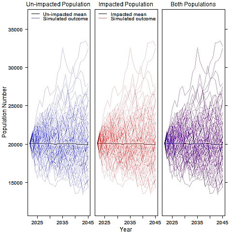
Figure 3.20: Minke Whale Scenario 4: Cumulative Projects, 1% Conversion Factor, no Vulnerable Subpopulation
3.4. Grey Seal
- There appears to be negligible alteration to the growth trajectory of grey seal, regardless of which of the conversion factor scenarios were explored for the Proposed Development alone ( Figure 3.21 Open ▸ , Figure 3.22 Open ▸ , Figure 3.23 Open ▸ ). Comparison of the size of the unimpacted population to the impacted population for all three scenarios showed no difference in the number of animals with the median of the ratio predicted to be 100% at all time points and for all scenarios. Given these very small changes there is not considered to be a potential for long term effects on this species as the difference falls within the natural stochasticity of the modelled population.
- Similarly for the cumulative scenario assessed within the north-east of Scotland no impacts were predicted on the population of grey seals, resulting from disturbance due to cumulative piling events ( Table 3.4 Open ▸ , Figure 3.24 Open ▸ ). This is not unexpected as both Seagreen 1A and Inchcape will finish piling prior to the commencement of piling at the Proposed Development so would not lead to a larger number of animals affected at any one time.
Table 3.4: Population Trajectory of Grey Seal Showing the Mean and Upper and Lower Confidence Limits at Different Time Points (Years After the Year in Which Piling Commences)
Figure 3.21: Grey Seal Scenario 1: 10% Reducing to 1% Conversion Factor, no Vulnerable Subpopulation
Figure 3.22: Grey Seal Scenario 2: 1% Constant Conversion Factor, no Vulnerable Subpopulation
Figure 3.23: Grey Seal Scenario 3: 4% Reducing to 0.5% Conversion Factor, no Vulnerable Subpopulation
Figure 3.24: Grey Seal Scenario 4: Cumulative Projects, 1% Conversion Factor, no Vulnerable Subpopulation
3.5. Harbour Seal
- There appears to be negligible alteration to the growth trajectory of harbour seal, regardless of which of the conversion factor scenarios were explored. Comparison of the ratio of unimpacted population to the impacted population for all three scenarios showed no difference ( Table 3.5 Open ▸ ).
- Results of the iPCoD modelling for harbour seal using the maximum adverse scenario 10% reducing to 1% scenario for the MU population (Scenario 1) show that the median of the ratio of the mean impacted population to the unimpacted population was one at four years (coinciding with the end of the first two piling campaigns) onwards until the maximum 25 year time point ( Table 3.5 Open ▸ , Figure 3.25 Open ▸ ). Therefore, there is not considered to be a potential for long-term effects on this species. These results were the same when using the 1% conversion factor scenario for the MU population (Scenario 2, Figure 3.26 Open ▸ ), and the 4% reducing to 0.5%conversion factor scenario for the MU population (Scenario 3, Figure 3.27 Open ▸ ), with the mean impacted population the same as the mean unimpacted population at time point 25. Since there is no discernible difference between the impacted and unimpacted populations there is therefore not considered to be a potential for any long-term effects on this species.
- Similarly for the cumulative scenario assessed within the north-east of Scotland no impacts were predicted on the population resulting from disturbance due to cumulative piling events ( Table 3.5 Open ▸ , Figure 3.28:). This is not unexpected since both Seagreen 1A and Inchcape will finish piling prior to the commencement of piling at the Proposed Development so would not lead to a larger number of animals affected at any one time.
Table 3.5: Population Trajectory of Harbour Seal Showing the Mean and Upper and Lower Confidence Limits at Different Time Points (Years After the Year in Which Piling Commences)
Figure 3.25: Harbour Seal Scenario 1: 10% Reducing to 1% Conversion Factor, no Vulnerable Subpopulation
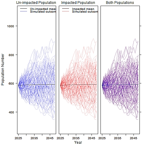
Figure 3.26: Harbour Seal Scenario 2: 1% Constant Conversion Factor, no Vulnerable Subpopulation
Figure 3.27: Harbour Seal Scenario 3: 4% Reducing to 0.5% Conversion Factor, no Vulnerable Subpopulation
Figure 3.28: Harbour Seal Scenario 4: Cumulative Projects, 1% Conversion Factor, no Vulnerable Subpopulation