Correction for availability bias 

85. In wildlife surveys, a proportion of seabirds that spend time underwater, especially while feeding, will not be detectable at the surface. This “availability bias” leads to an under-estimate of their abundance.
86. Barlow et al. (1988) produced a method to estimate true abundance by using correction factors based on species-specific data on time spent underwater.
87. Following Barlow et al. (1988) the probability that an animal is available at the surface is calculated as:

Where s is the average time spent at the surface, t is the window of time that the animal is within view and d is the average time below the surface. In the case of digital video surveys, the value of t is negligibly small and is treated as 0.

88. Using Barlow’s method, we calculated the proportion of time that an animal was available at the surface (Pr (visible)) for guillemot and razorbill. Absolute density, corrected for availability, was then obtained by dividing the density of birds observed by the Pr(visible).
89. For guillemots and razorbills, data obtained during the breeding season using data loggers was used to estimate availability bias. Thaxter et al. (2010) give mean times for these species engaged in flying, feeding and underwater per trip during the chick-rearing period.
90. Thus, the proportion of time that guillemots and razorbills were available at the surface (Pr(visible)) was estimated at 0.7595 and 0.8182, respectively.
91. For puffins the results from a study using data loggers reported in Spencer (2012) were used. The results show that puffins spend 14.16% of daylight time underwater. This infers that the proportion of time that puffins were available at the surface (Pr(visible)) was 0.8584.
92. The estimates of Pr(visible) for guillemots, razorbills and puffins were used to correct relative abundance estimates of birds sitting on the sea. These corrected abundance estimates for sitting birds were then added to the abundance estimate of flying birds to give an overall absolute abundance for each species.
93. Correction for availability bias was not undertaken for any other species due to a lack of information about diving patterns.

3.2.7.    Consideration of biological seasons

94. Bird abundance and distribution varies greatly throughout the year, dictated largely by season and bird biology. This report recognises two main biologically distinct ‘bio-seasons’, which aid in understanding the importance of the site for each species during a yearly cycle. We have used the seasonal definitions outlined in NatureScot guidance (2020a), as agreed during the Ornithology Road Map process. Seasonality is complex and periods differ between species based on life history traits, with timings an approximation. Figures collated for each species are summarised in Figure 3.6   Open ▸ . Bio-seasons used within this technical baseline report are:

• Breeding season: birds are strongly associated with a nest site, including nesting, egg-laying and provisioning young.
• Non-breeding season: period where no breeding takes place, which may encompass birds over-wintering in an area and migration periods between breeding and wintering sites dependent on the species.

Figure 3.6:    Gantt chart of species-specific bio-seasons used in this report, adapted from NatureScot (2020a) including the breeding season (green), non-breeding (blue) and pre-breeding (orange)

3.2.8.    Calculation of Mean Seasonal Peaks

95. Mean seasonal peak (MSP) population estimates were calculated for each species in each bio-season, taken as an average over the two years of surveying (March 2019 – April 2021). For example, the MSP population estimate for the breeding season was calculated as the average of the peak count in the breeding season in year one and the peak count in the breeding season in year two.

96. Surveys were generally assigned to a season based on the day of the month that the survey was flown. For seasons starting or ending halfway through the month, the 15/16 was used as a mid-month cut off. This was necessary to avoid the same monthly estimate potentially being used in both the breeding and non-breeding season.
97. To account for months where there was no survey, some flights were assigned to different months or years to ensure coverage of all months in both seasons for a two-year period ( Table 3.2   Open ▸ ). The Applicant discussed this allocation during the Ornithology Road Map process (RM4) and followed subsequent joint advice from Marine Scotland and NatureScot received through email on 14 January 2022.
98. This treatment of surveys was only conducted for calculation of mean-seasonal peaks and age class proportions, with all other data presented in this technical report by the date that the surveys were flown.

Table 3.2   Open ▸ :  Treatment of rescheduled surveys for calculation of mean seasonal peaks (MSPs) and age proportions per season

99. MSP population estimates are presented for the offshore Ornithology Study area for context. MSPs for the for the Development array plus a 2km buffer, which are required for relevant species for displacement modelling and assessment are also reported. MSPs for the array area only are reported separately in the Appendix 11:4: Ornithology Displacement Technical Report.

3.2.9.    Calculation of Age Class Proportions

100. To assess the proportion of birds in each age class (adult, immature, juvenile), the average or mean number of birds recorded in each class was calculated across all surveys that occurred in each season. For example, if there were four surveys in the breeding season in year one and four surveys in the breeding season in year two, then the average number of adult birds was calculated across eight surveys in total. This was conducted using all data within the 16 km boundary. Surveys were assigned to a season based on the day that the survey was flown, with the exceptions listed in Table 3.2   Open ▸ . For seasons starting or ending halfway through the month, the 15/16 was used as a mid-month cut off.
101. The resulting proportion in each class was calculated as a proportion of the sum of the average number in each age class. This is presented for species where aging was possible, namely gulls, gannets and terns.

4. Results

102. The total number of birds observed during the 25 surveys in the Offshore Ornithology Study Area and subsequently identified to species level are presented in Table 4.1   Open ▸ and Table 4.2   Open ▸ . Species addressed in greater detail within this report are highlighted in grey. Birds which could not be identified to species level but were assigned to a broader species group are presented in Table 4.3   Open ▸ and Table 4.4   Open ▸ . For comparative purposes between survey years, all species recorded are presented in Table 4.1   Open ▸ and Table 4.2   Open ▸ , even if only recorded in one year.
103. Scientific names of species and taxonomic groupings are presented in Annex A.

Table 4.1:  Raw counts of birds detected and assigned to species level in Year 1 of surveying at Offshore Ornithology Study Area: March 2019 to February 2020

Table 4.2:  Raw counts of birds detected and assigned to species level in Year 2 of surveying at Offshore Ornithology Study Area: March 2020 to April 2021

Table 4.3:  Raw counts of birds with no species ID, assigned to species groups, in Year 1 of surveying at Offshore Ornithology Study Area: March 2019 to February 2020

Table 4.4:  Raw counts of birds with no species ID, assigned to species groups, in Year 2 of surveying at Offshore Ornithology Study Area: March 2020 to April 2021

4.1. Abundance estimates: comparison of design- and model- based

104. Plots of density and associated 95% confidence intervals for each survey for kittiwake, guillemot, razorbill, puffin and gannet enable comparison between estimates generated from design and model-based methods.
105. Kittiwake estimates were relatively similar from the two methods throughout the study period ( Figure 4.1   Open ▸ ). Likewise, for razorbill and puffin, the estimates from the two methods were effectively the same, as demonstrated by the overlapping confidence intervals ( Figure 4.3   Open ▸ and Figure 4.4   Open ▸ respectively).
106. Estimates produced by both methods for gannets were similar apart from December 2019 and February 2020, where MRSea produced much larger population estimates. This was due to the model being unable to resolve the spatio-temporal relationship in the survey gaps, leading to unrealistic estimates.
107. The estimates using design-based and MRSea methods for guillemots were relatively similar. However, in October 2019 MRSea produced a significantly higher estimate than those produced by the design-based method. There was also less variation in the two methods outputs in Year 2 (2020/21) ( Figure 4.2   Open ▸ ).
108. MRSea results cannot be replicated despite reruns with the same code and input parameters as the stochasticity in the bootstrapping used to produce estimates will lead to different values on every run and due to the selection of spatial knots.
109. The use of density-based estimates was more appropriate for downstream processes due to the instability of MRSea across several metrics. First, confidence limits of model-based population estimates were wider than design-based in most cases, particularly in October 2019 surveys. An often-cited desirable trait of model-based estimates is the ability to generate tighter confidence limits around population estimates. However, design-based estimates provided tighter confidence limits compared to model-based estimates in this case. Another reason for the selection of design-based over model-based population estimates was related to stochasticity in the MRSea process which generated vastly different results when running the same set of code with no changes in data or parameters ( Table 4.5   Open ▸ and Table 4.6   Open ▸ ). This seemed to be related to the random selection of spatial knots combined with large gaps in the survey areas. This stochasticity meant that the MRSea results were unreliable (in April S02 of the 2021 surveys, there was a difference of 2,438 individuals between both model runs, while in October 2019, due to large gaps in survey effort, in one model, the mean estimate was unrealistically high, while in the next run, estimates were in line with other months). Although the estimates fall within respective confidence limits between runs, the differences would invariably impact MSPs used for displacement and, for other species, density estimates for collision risk modelling.
110. On a technical point, another reason for using design-based estimates rather than the MRSea outputs was because of the inability to save output files from MRSea to allow for re-examination of model outputs. File sizes of the outputs were on the order of 20 GB (due to the size of the dataset) and were unable to be re-read into the R interface, meaning re-visiting models was not possible. This issue was raised at the Marine Scotland Ornithology Impact Assessment Workshop on the 22 February 2022, and it was confirmed that there are currently no plans to change output file format. The possibility of modelling at a monthly scale (as opposed to a seasonal scale; suggested by Scott-Hayward during the Marine Scotland Ornithology Impact Assessment Workshop) to help overcome issues with data gaps was not considered because downstream processes required population estimates at the survey-level scale to aggregate data.
111. Annex L provides monthly population estimates by species from the MRSea analyses and spatial maps of the mean densities and uncertainty (95% CIs and CVs) around those estimates.

Table 4.5:  Exemplar abundance outputs from two runs of MRSea for guillemot from March 2019 to February 2020. Input data and model parameters were identical with the only difference being between location of the spatial knots

Table 4.6:  Exemplar abundance outputs from two runs of MRSea for guillemot from March 2020 to April 2021. Input data and model parameters were identical with the only difference being between location of the spatial knots

Figure 4.1:  Comparison of the density estimates produced using design-based and MRSea methods for kittiwakes

Figure 4.2:  Comparison of the density estimates produced using design-based and MRSea methods for guillemots

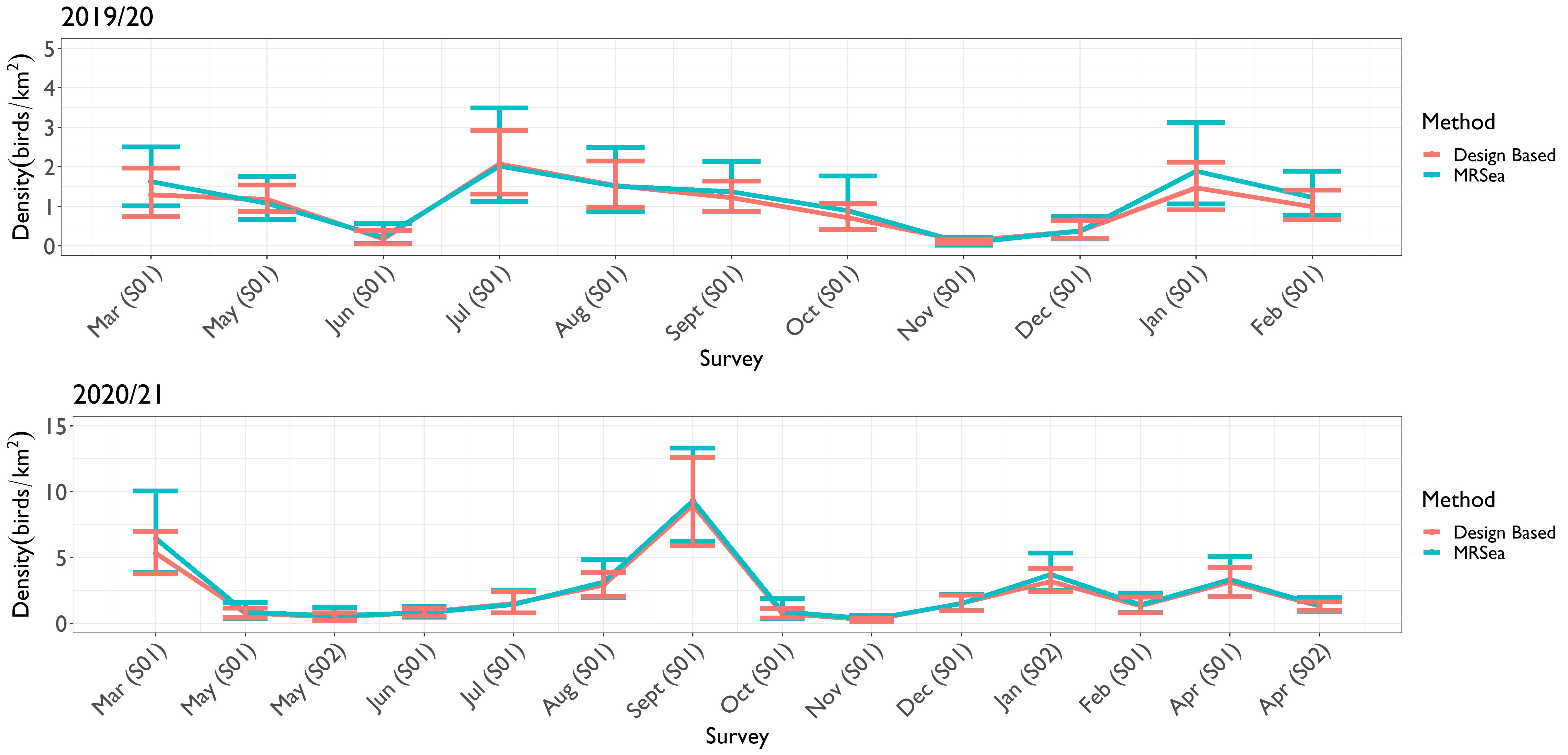
Figure 4.3:  Comparison of the density estimates produced using design-based and MRSea methods for razorbills

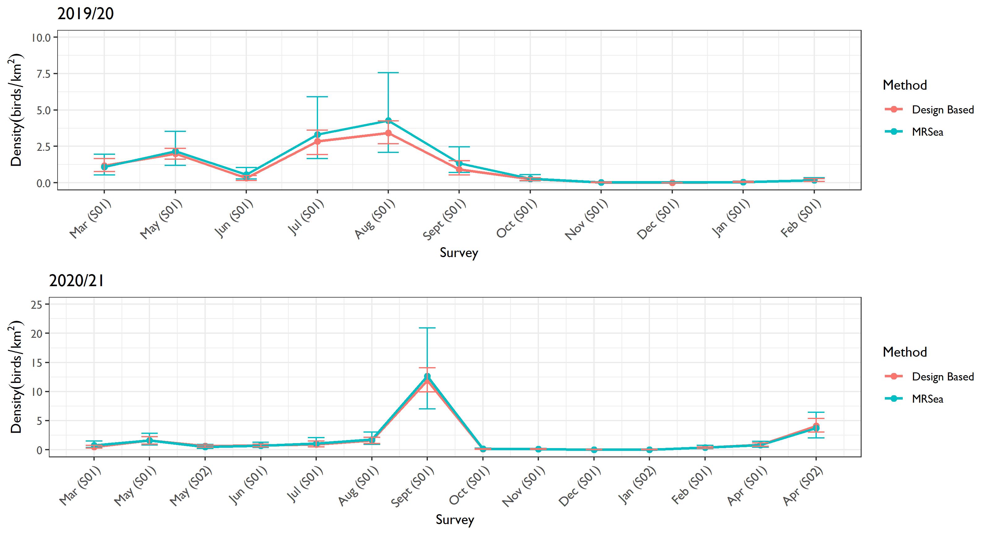
Figure 4.4:  Comparison of the density estimates produced using design-based and MRSea methods for puffins

Figure 4.5:  Comparison of The Density Estimates Produced Using Design-Based and Mrsea Methods for Gannets

5. Species accounts

112. Eighteen species are the focus of the species accounts and discussed in greater detail below:

• common scoter;
• kittiwake;
• black-headed gull;
• little gull;
• common gull;
• herring gull;
• lesser black-backed gull;
• common tern;
• arctic tern;
• great skua;
• guillemot;
• razorbill;
• puffin;
• gannet;
• red-throated diver;
• fulmar;
• manx shearwater; and
• shag.

113. These species were identified taking account of the Berwick Bank Scoping and HRA Screening Reports, and ensure relevant information is provided for Environmental Impact Assessment.
114. For each species account, estimates are provided for the Offshore Ornithology Study Area, apportioned for unidentified birds and adjusted for availability bias where appropriate. Unapportioned estimates, and those for the Project only, are provided in the attached annexes (see Table 5.1   Open ▸ ). Population estimates for a 2 km buffer around the Project are presented separately in Appendix 11.4: Ornithology Displacement Technical Report.
115. Low densities may appear as 0.00 birds/km2 yet still have low population estimates presented. This is simply a result of rounding very low densities to 2 decimal places. Similarly, some upper confidence limits presented in graphs may appear to sit at the mean; this is also an issue of rounding.

Table 5.1:    Summary of content of Annexes A to L. Dev array= Development array. ‘Apportioned?’ Refers to whether the estimates are for all birds, including those detections assigned to a species group but latterly assigned to a species

*Estimates presented on a survey-by-survey basis, rather than grouped by species

5.1. Kittiwake

116. The most abundant gull species globally, kittiwakes are small coastal seabirds which form large colonies during the breeding season, before dispersing offshore for the non-breeding season (Mitchell et al., 2004; Coulson, 2011). Many large colonies are located along the east coast of Scotland, although some are also present on man-made structures such as buildings and oil rigs (Mitchell et al., 2004). The species is currently Red-listed on the UK Birds of Conservation Concern List (Stanbury et al., 2021).
117. Kittiwake productivity (defined by mean fledged chicks per nest) increased along the east coast of Scotland between 2009 and 2019. Although sea surface temperature (SST) increased in the Firth of Forth 1980-2010, the following decade saw a decrease in sea surface temperature (SST) in the region and this is thought to have had a positive effect on productivity (Wanless et al., 2018; JNCC, 2021). Consequently, abundance and breeding success have shown a degree of stability over the period 2011 – 2018 for many of the key species, including kittiwake (Scotland’s Marine Assessment, 2020).
118. It is likely that decreases in SST positively influence sandeel abundances, increasing the availability of this food source to kittiwakes within the region (Arnott and Ruxton, 2002). Kittiwakes are particularly vulnerable to changes in sandeel availability (Frederiksen et al., 2005), as birds can only feed at or near the sea surface, thus having less access to a greater range of species in the water column. Kittiwake productivity and survival was previously affected by a sandeel fishery in south-east Scotland, which ceased operation in 2000 (Frederiksen et al., 2004).
119. Estimated apportioned densities from design-based analysis ranged between 0.48 (November 2019) and 13.86 (September 2020) birds/km2, equating to population estimates for the Offshore Ornithology Study Area ranging between 1,903 birds (95%CI 1,031 – 3,128; November 2019) and 55,139 birds (95%CI 41,872 – 71,811; September 2020) ( Table 5.3   Open ▸ ).
120. High abundances of kittiwakes within the Offshore Ornithology Study Area in summer months, such as August 2019 and 2020 ( Table 5.3   Open ▸ ), are consistent with Berwick Bank and Seagreen boat-based seabird surveys, where kittiwakes accounted for a high proportion of the total birds present, calculated at 23.67%, 24.80% and 21.60% of all detections respectively. Analysis of ESAS data by Kober et al. (2010, 2012) indicated the outer Firth of Forth is likely to be most important for kittiwakes during the breeding season. The total count of kittiwakes within the foraging range (mean max distance +1 sd from Woodward et al. 2019) of the Project approximates the regional population and is estimated at 319,126 breeding adults.  
121. Egg-laying typically occurs between May and early June (Coulson, 2011); and this is reflected in decreased kittiwake abundance in the Offshore Ornithology Study Area as adult birds are in attendance at colonies. Chicks hatch through June and July and rearing continues until juveniles fledge six weeks later. Use of the Offshore Ornithology Study Area whilst foraging may occur during chick-rearing, but generally the highest abundances were recorded in late summer, such as in August 2019 and August/September 2020, coupled with high proportions of juvenile birds at this time ( Table 5.3   Open ▸ ; Table 5.8   Open ▸ ). These results indicate that the Offshore Ornithology Study Area is primarily used by post-fledging kittiwakes before dispersal to wintering areas. High incidence of kittiwakes within the breeding season is also consistent with data collected during the IMPRESS project (Camphuysen, 2005). Relatively high abundance recorded in March 2019 may be attributed to the movement of birds to breeding colonies prior to egg laying.
122. Mean seasonal peak population estimates indicate the Offshore Ornithology Study Area is important for the species during the non-breeding season, with design-based analysis estimating approximately 50,958 birds (95%CI 35,530 – 69,349) ( Table 5.6   Open ▸ ). Mean-peak estimates for the breeding season remain high, calculated at 36,189 birds (95%CI 24,774 – 49,254). Relatively high abundances right after the breeding season (e.g. September 2020) are likely to have led to the non-breeding mean seasonal peak, with abundance being generally low throughout this period until the start of the breeding season.
123. Behaviour differed between seasons ( Figure 5.6   Open ▸ ), with the largest proportions of flying birds generally occurring between April and June, and October and December dependent on year. These peaks in flying activity generally coincided with the start and end of the breeding season, with a peak of 86% (197 birds) recorded flying in November 2019. Large proportions of birds were recorded as sitting on the water in most surveys, indicative of recent feeding activity, suggesting the Offshore Ornithology Study Area is used for foraging year-round. The highest proportions of sitting birds generally occurred in spring and mid to late summer, coinciding with the breeding season. This reaffirms the possibility that birds are congregating in the area prior to the breeding season and may be feeding in the area during or after chick-rearing. High proportions of sitting birds (75%) were also recorded in February 2021.
124. The largest average proportion of juveniles (11% of aged birds) coincided with the non-breeding period; the same was true for immature birds (7% of aged birds; Table 5.8   Open ▸ ).
125. Flight direction varied considerably between months and bio-seasons ( Figure 5.5   Open ▸ ). In September 2020, when the highest densities of kittiwakes were estimated, birds primarily flew southwest, however, in March 2019 when high densities were also present, many kittiwakes also flew southwards. In April S01 2021, many birds flew north and south, with few birds flying east or west.  

Table 5.2:   Kittiwake bio-seasons taken from NatureScot (2020a)

Table 5.3:  Monthly density and population estimates of all kittiwakes across the Offshore Ornithology Study Area using design-based analysis. Data include “no-identification” birds apportioned to species

Table 5.4:  Monthly density and population estimates of flying kittiwakes only across the Offshore Ornithology Study Area using design-based analysis. Data include “no-identification” birds apportioned to species

Table 5.5:  Monthly density and population estimates of sitting kittiwakes only across Offshore Ornithology Study Area using design-based analysis. Data include “no-identification” birds apportioned to species

Figure 5.1:  Estimated densities (birds/km2) of all kittiwakes across the Offshore Ornithology Study Area using design-based analysis. Data include “no-identification” birds apportioned to species

Table 5.6:  Mean seasonal peak (MSP) population and density (birds/km2) of all kittiwakes in the Offshore Ornithology Study Area across the two years of surveying (March 2019 to April 2021) estimated using design-based analysis. Data include “no-identification” birds apportioned to species

Table 5.7:  Mean seasonal peak (MSP) population and density (birds/km2) of all kittiwakes in the Berwick Bank Development Array plus 2km buffer across the two years of surveying (March 2019 to April 2021) estimated using design-based analysis. Data include “no-identification” birds apportioned to species

Figure 5.2:  Distribution of kittiwakes across the Offshore Ornithology Study Area between March 2019 and March 2020

Figure 5.3 Distribution of kittiwakes across the Offshore Ornithology Study Area between May S01 2020 and April S01 2021

Figure 5.3 Distribution of kittiwakes across the Offshore Ornithology Study Area between May S01 2020 and April S01 2021

Figure 5.3  Distribution of kittiwakes across the Offshore Ornithology Study Area between May S01 2020 and April S01 2021

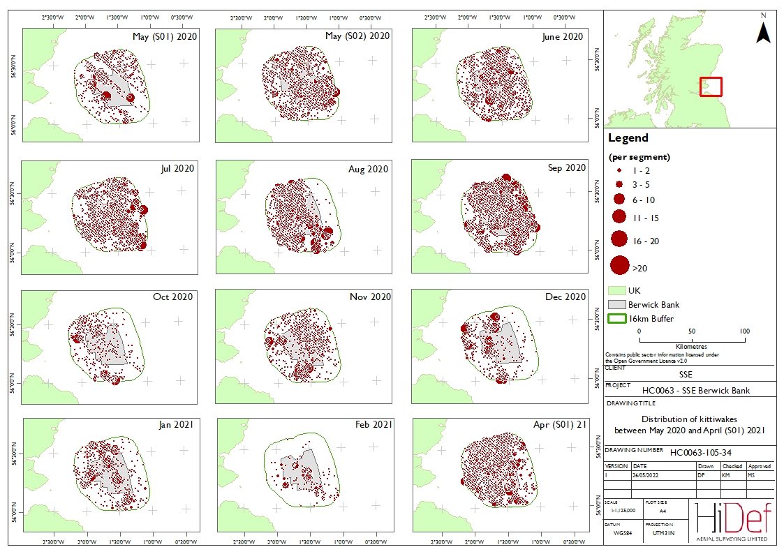
Figure 5.4:  Distribution of kittiwakes across the Offshore Ornithology Study Area in April S02 2021

Table 5.8:   Mean count, SD and proportion of kittiwakes in each age class averaged across bio-season

Figure 5.5:  Summarised flight direction of kittiwakes across the Offshore Ornithology Study Area

Figure 5.6:  Percentage of flying kittiwakes per survey across the Offshore Ornithology Study Area

5.2. Guillemot

126. One of the most abundant seabird species in the northern hemisphere, in the breeding season, guillemots are generally found in coastal colonies consisting of up to tens of thousands of individual birds (Mitchell et al., 2004). Typically, only coming to coastal areas to breed, most birds move offshore during the non-breeding season (Wernham et al., 2002). As pursuit divers, guillemots generally feed on schooling fish such as cod and sprat (Gaston and Jones 1998), however this is likely to differ depending on local feeding conditions (Merkel, 2019). Large breeding colonies in proximity to the Offshore Ornithology Study Area are present on the Isle of May and St Abb’s Head with approximately 18,705 and 42,905 individuals recorded in 2018 respectively (SMP, 2021). The species is currently Amber-listed on the UK Birds of Conservation Concern List (Stanbury et al., 2021).
127. Guillemots were the most abundant species recorded in the Offshore Ornithology Study Area during the survey programme, with birds recorded most frequently between April and May and August and/or September in both years, coinciding with the start of the breeding season and the post-breeding flightless moult stage ( Table 5.10   Open ▸ ). Evidence suggests guillemots may be present in large aggregations post-breeding along the east coasts of Scotland and England, coinciding with high local prey abundance (Furness, 2015). Aggregations are likely to be highly dependent on prey availability, lasting only two to three weeks. Movement down the east coast of Scotland from the northern North Sea during post-breeding migration and dispersal has also been indicated (Figure 21.3; Furness, 2015), with spring migration expected to occur in the opposite direction (movement of breeding birds northwards along the Scottish east coast). Density estimates produced using design-based methods ranged between 2.12 birds/km2 (95%CI 1.35 – 3.22; November 2019) and 60.88 birds/km2 (95%CI 47.69 – 76.93; April S02 2021) over the entire survey period, when adjusted for availability bias.
128. Peak population estimates in April S02 2021 equated to 242,168 birds (95%CI 190,509 – 305,941). The total count of guillemots at SPAs within foraging range (mean max distance +1 sd from Woodward et al. 2019) of the Project approximates the regional population and is estimated at 353,971 breeding adults. There are other large colonies, such as the 148,805 breeding adults at North Caithness Cliffs SPA, which may also frequent the Firth of Forth region based on modelled tagging data (Wakefield et al. 2017, 2019). The relatively high abundance estimated for the site in April S02 2021 is likely to be explained by a good breeding season in 2020 (supported by our data for September 2020 and NatureScot, 2021), which as a consequence will lead to a high number of birds returning to the area ahead of the following 2021 breeding season. As the most recent SPA counts used were from 2014 to 2019, except for Forth Islands SPA which includes counts up to 2021, the successful breeding season observed in 2020 will not be reflected in the SPA estimated totals for guillemot. A pattern emerges where the number of birds seen in March/April is predicated (to a large extent) by the success of the breeding season in the previous year; this pattern is seen in the Year 1 data, where the breeding/post breeding peak abundance estimates are lower (August 19) than the pre/breeding season return of guillemot to the area to access the colonies the following year (May SO1 20 as “April”).
129. Data collected from boat-based surveys of the Berwick Bank and Seagreen in 2020 and 2021 also recorded an abundance of guillemots, with the species making up the largest proportion of all recorded birds (32.09%, 28.10% and 29.30% respectively). Camphuysen et al. (2004) reported a decline in breeding success within the outer Firth of Forth between 1997 and 2003. However, since 2007, this trend has reversed and breeding success recovered to a high level in the 2010s (Harris et al., 2017).
130. Overall, guillemots were recorded in higher densities in Year 2 compared to Year 1, with design-based density estimates ranging between 2.12 birds/km2 (95%CI 1.35 – 3.22) and 40.26 birds/km2 (95%CI 27.91 – 54.40) in 2019/20 compared to 4.82 birds/km2 (95%CI 3.74 – 5.92) and 60.88 birds/km2 (95%CI 47.89 – 76.93) in 2020/21. After the post-breeding peak, abundance declines substantially, likely due to dispersal offshore to the North Sea after chick-rearing (Wernham et al., 2002; Forrester et al., 2007). When accounting for availability bias, estimates of density were higher during the breeding season, with mean peak densities for the region estimated at 46.91 birds/km2 (95%CI 37.98 – 57.83), compared to 34.88 birds/km2 (95%CI 27.41 – 43.02) during the non-breeding season ( Table 5.13   Open ▸ ).
131. High guillemot abundance in the breeding season coincides with the onset of egg-laying and incubation (Harris and Wanless, 2004). During this time, most birds were recorded as sitting on the water, which is to be expected considering their feeding strategy of diving from the water surface. A high proportion of sitting birds were also observed during the secondary peaks between August and September, likely due to the presence of many flightless adult birds which moult after the chick-rearing period (Brown and Grice, 2005). As expected, extremely low percentages of flying birds were present within the population at this time ( Figure 5.12   Open ▸ ) and consequently a lack of flight direction data for guillemots in August and September in both 2019 and 2020 ( Figure 5.11   Open ▸ ).  
132. Overall, flight direction data indicated guillemots generally flew in easterly and westerly directions such as in March 2019 and between March and May 2020, with May 2019 being the only month in which a large proportion of birds flew south ( Figure 5.12   Open ▸ ). Movement east and west may be attributed to adult birds moving between nest sites to the west of the Offshore Ornithology Study Area such as the Isle of May and Craigleith and foraging grounds further offshore in the outer Firth of Forth and North Sea (Furness, 2015).
133. Ages of birds are not presented for this species since adults can only be aged when in the presence of a juvenile for size comparison, and they almost exclusively occur as single adult-chick pairs.

Table 5.9:   Guillemot bio-seasons taken from NatureScot (2020a)

Table 5.10:  Monthly absolute density and population estimates of all guillemots across the Offshore Ornithology Study Area using design-based analysis, adjusted for availability bias. Data include “no-identification” birds apportioned to species

Table 5.11:  Monthly density and population estimates of all flying guillemots only across the Offshore Ornithology Study Area using design-based analysis. Data include “no-identification” birds apportioned to species

Table 5.12:  Monthly absolute density and population estimates of sitting guillemots only across the Offshore Ornithology Study Area using design-based analysis, adjusted for availability bias. Data include “no-identification” birds apportioned to species

Figure 5.7:  Estimated absolute densities (birds/km2) of all guillemots across the Offshore Ornithology Study Area using design-based analysis, accounting for availability bias. Data include “no-identification” birds apportioned to species

Table 5.13:  Mean seasonal peak (MSP) population and density (birds/km2) of all guillemots in the Offshore Ornithology Study Area across the two years of surveying (March 2019 to April 2021) estimated using design-based analysis, with figures adjusted for availability bias. Data include “no-identification” birds apportioned to species

Table 5.14:  Mean seasonal peak (MSP) population and density (birds/km2) of all guillemots in the Berwick Bank Development Array plus 2 km buffer across the two years of surveying (March 2019 to April 2021) estimated using design-based analysis, with figures adjusted for availability bias. Data include “no-identification” birds apportioned to species.

Figure 5.8:  Distribution of guillemots across the Offshore Ornithology Study Area between March 2019 and March 2020

Figure 5.9:  Distribution of guillemots across the Offshore Ornithology Study Area between May S01 2020 and April S01 2021

Figure 5.10:   Distribution of guillemots across the Offshore Ornithology Study Area in April S02 2021

Figure 5.11:   Summarised flight direction of guillemots across the Offshore Ornithology Study Area

Figure 5.12:  Percentage of flying guillemots per survey across the Offshore Ornithology Study Area